In my most recent published paper, I analysed the effects of incoming solar UV-B radiation on the geochemistry of Atlas cedar pollen, focused on the Middle Atlas Mountains in Morocco. The study area was relatively small, with sample sites fairly close together.
The UV-B data was obtained from the glUV: Global UV-B radiation dataset, which combines data from NASA's Ozone Monitoring Instrument (OMI) onboard the Aura spacecraft, into grid cells containing average erythemally weighted estimates of daily UV-B radiation. You can read full details of the methods used in the associated research paper (Beckmann et al. 2014) (Available open access).
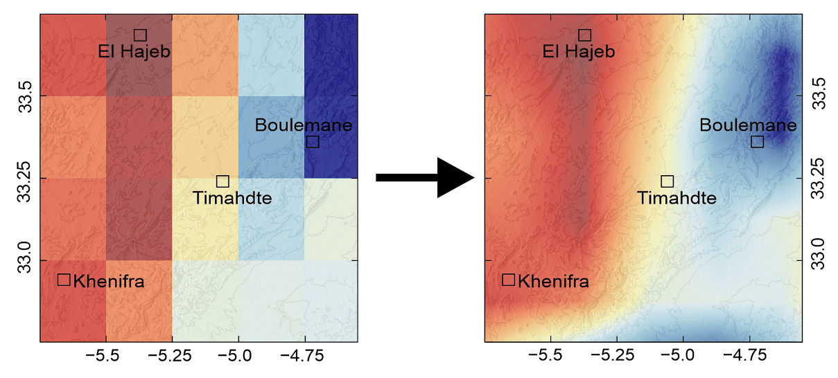
Gridded datasets are an excellent source of data for doing global or macro-scale studies. However, if working in a relatively small area, you may find that your study area is covered by just a few grid cells due to the often low resolution of gridded data. And this can sometimes make it more difficult to carry out analysis.
To overcome the problem, you can interpolate the data to increase the resolution. After interpolation, the gridded data will go from looking like the image on the left, to looking like the image on the right, which is much more detailed for the study area.
Read on to find out how to do this in R!
Guide Information
| Title | Interpolating gridded datasets in R: UV-B data |
| Author | Benjamin Bell |
| Published | June 19, 2018 |
| Last updated | |
| R version | 3.5.0 |
| Packages | base; raster |
| Navigation |
Overview
Gridded datasets are available for all kinds of data, particularly for climate data (see my previous blog post for getting climate data). They are available in different resolutions, and usually cover the entire planet.
In this guide, I will show you how to interpolate gridded data using bilinear interpolation with the "raster" package in R. The example will use gridded UV-B data from the glUV dataset, available in ASCII format.
You can also use this guide to interpolate other kinds of gridded data (e.g. CRU climate data), although I will publish a separate step-by-step guide for doing this in a future blog post.
Getting the data
You can download the UV-B data from the glUV: Global UV-B radiation dataset website. Click on the Download link on the left to see the available datasets. For this guide, we'll use the Monthly Mean UV-B dataset for the Month of August. To download, right-click on the link that says "August (16 MB)" and save the file to your computer.

The UV-B data file is in the ASCII format, which is essentially a text file that can be read by almost any text editor. Here is how the data looks in Notepad++

There is some important information contained within the file. The NCOLS and NROWS values refer to how many rows and columns make up the grid. The XLLCORNER and YLLCORNER refer to decimal degrees coordinates, and indicate where the grid starts. The CELLSIZE refers to the size of the grid cells in degrees. In this case, each cell represents an area 0.25° squared. This is equivalent to approximately 27.5 km2. The NODATA_value refers to the value where no data is available for that grid cell. In this case, if a grid cell contains "-9999", then no UV-B data is available.
The UV-B values in this dataset are in J/m2/day. I.e. the values represent the average UV-B dose per day (in Joules per metre squared), averaged over a month.
Importing the data into R
The benefit of ASCII files, is that they can be easily read by many programs, including R. To import this dataset into R, we'll make use of the "raster" package. If you do not already have this package installed, use install.packages("raster") to install it from within the R console.
To import the data, you should save the file to the R working directory, and then use the following code:
# Load library
library(raster)

# Import UV-B data into R
uvb8 <- raster("56472_glUV_August_monthly_mean.asc")
(You will need to adjust the code if you have downloaded the UV-B data to a different file location).
If you type "uvb8" into the R console, you'll be presented with information about the data:
> uvb8
class       : RasterLayer
dimensions  : 720, 1440, 1036800  (nrow, ncol, ncell)
resolution  : 0.25, 0.25  (x, y)
extent      : -180, 180, -90, 90  (xmin, xmax, ymin, ymax)
coord. ref. : NA
data source : 56472_glUV_August_monthly_mean.asc
names       : X56472_glUV_August_monthly_mean
Here, you can see the dataset consists of 1,036,800 values which cover the planet. You could also plot this data to visualise it:
plot(uvb8)

You can just about make out the shape of the different continents on this plot.
After importing the data into R, you will now be able to manipulate it.
Interpolating gridded data
Setting an extent
Before we interpolate the data, we first need to subset the data to cover the study area. In this example, we will be looking at the Middle Atlas Mountains, and the surrounding area in Morocco.
So, we need to create an "extent" - this tells R the coordinates of the area that we would like to subset the data for. For the Middle Atlas area, you can set the extent using the following code:
# Set Middle Atlas Extent (interpolation area)
midatlas <- extent(c(-8, -2, 30, 36))
You can change the coordinates to different values depending on your own study area. The coordinates should be input using decimal degrees, where the first and second numbers represent the longitude (xmin, xmax), while the third and fourth numbers represent latitude (ymin, ymax).
It is generally a good idea to create a slightly bigger extent than your study area. E.g. add at least 1° to the xmin, xmax, ymin, ymax values.
Also, as we'll be using bilinear interpolation, it is important that the area we subset (i.e. the extent) is a square, containing an equal number of grid cells on each axis. If using a different interpolation method, this is less important.
If you do not know the coordinates to set the extent, it is possible to draw the extent on the map using the drawExtent() function, using the following code:
# Plot map
plot(uvb8)
# Draw extent
drawExtent()
This will start an interactive session - you should now click on the plot to draw your extent. The first click should be the xmin, and the second click should be the ymax. (The best thing to do, is to play around, clicking on the map to understand how this works).

R will then output the coordinates in the R console:
> drawExtent()
class       : Extent
xmin        : -18.75498
xmax        : -2.875476
ymin        : 25.03412
ymax        : 33.61764
(Your values will differ).
Once you have set the extent, you can then subset the data:
# Subset the UV-B data to the Middle Atlas area
uvb8.ex <- extract(uvb8, midatlas, ncol=24)
In this code, we create a new object (uvb8.ex) which contains the UV-B data we imported earlier for our study area (the midatlas extent).
The ncol=24 argument tells R to create the new data grid with 24 columns. This value is important for the interpolation to work properly.
The extent in our example covers the longitude (x axis) from -8 to -2 on our map, which is equal to 6°. As the grid cells in the gridded dataset are 0.25° in size (4 grid cells for each 1°), this means that for our extent, there are 24 grid cells along the x axis (6 X 4 = 24). There are also 24 grid cells along the y axis, although it is not necessary to specify this here.
If you have used a different extent, or you have used a different resolution dataset, you will need to re-calculate the ncol value.
Bilinear interpolation
Bilinear interpolation in simple terms, will interpolate the gridded data in two directions. Firstly, it interpolates the data in one direction, and then does the same again in the other direction.
This is a "simple" method, which works particularly well for gridded data. There are many other interpolation methods available, which might be more suitable for your data.
Now that we have subsetted and extracted the UV-B data for the Middle Atlas region, we can go ahead and interpolate it.
First, we'll create a RasterLayer object with our subsetted data, which will become our "coarse" grid:
# Create RasterLayer using the subsetting UV-B data
ma.uvb8.c <- raster(ext=midatlas, vals=uvb8.ex, nrow=24, ncol=24)
This code tells R to create a new RasterLayer object (ma.uvb8.c) using the extent (midatlas), with the UV-B values we extracted (uvb8.ex), and it should be 24 by 24 cells in size.
You can verify that this has been done correctly by typing "ma.uvb8.c" into the R console:
> ma.uvb8.c
class       : RasterLayer
dimensions  : 24, 24, 576  (nrow, ncol, ncell)
resolution  : 0.25, 0.25  (x, y)
extent      : -8, -2, 30, 36  (xmin, xmax, ymin, ymax)
coord. ref. : NA
data source : in memory
names       : layer
values      : 4851.697, 6893.227  (min, max)
Next, we need to create a RasterLayer which has a "fine" resolution grid for our extent:
# Create fine resolution grid
ma.f <- raster(ext=midatlas, ncol=2400, nrow=2400)
This code will create an empty grid, with grid cells that are 100 times smaller than the original grid. (The smaller the grid cells, the higher the resolution).
You can adjust the resolution of the grid by changing the ncol and nrow values. You could for example increase the resolution by 1000. However, be warned, that increasing the resolution increases the amount of time, and the amount of memory needed by R to do the interpolation. You may be limited by your computer power as to what resolution you can use.
Again, you can verify the new RasterLayer grid by typing "ma.f" into the R console:
> ma.fc
class       : RasterLayer
dimensions  : 2400, 2400, 5760000  (nrow, ncol, ncell)
resolution  : 0.0025, 0.0025  (x, y)
extent      : -8, -2, 30, 36  (xmin, xmax, ymin, ymax)
coord. ref. : +proj=longlat +datum=WGS84 +ellps=WGS84 +towgs84=0,0,0
You can see that the resolution of this RasterLayer is much finer (i.e. the resolution has increased).
Lastly, you can perform the interpolation by resampling the coarse gridded data to the fine grid:
# Resample coarse grid to the fine grid
ma.uvb8 <- resample(x=ma.uvb8.c, y=ma.f, method="bilinear")
This code will create a new RasterLayer object (ma.uvb8), which will interpolate the data from the coarse grid (ma.uvb8.c) to the fine resolution grid (ma.f) using bilinear interpolation.
You can verify the interpolation has worked by typing "ma.uvb8" into the R console:
> ma.uvb8
class       : RasterLayer
dimensions  : 2400, 2400, 5760000  (nrow, ncol, ncell)
resolution  : 0.0025, 0.0025  (x, y)
extent      : -8, -2, 30, 36  (xmin, xmax, ymin, ymax)
coord. ref. : +proj=longlat +datum=WGS84 +ellps=WGS84 +towgs84=0,0,0
data source : in memory
names       : layer
values      : 4836.982, 6886.999  (min, max)
The RasterLayer should contain additional information (data source, names, values) which will indicate that the interpolation was successful. You could also plot the data to compare the original (non-interpolated) vs. the interpolated data:
# Plot original vs. interpolated data
layout(matrix(1:2, ncol=2))
plot(ma.uvb8.c)
plot(ma.uvb8)

Here, you can clearly see the interpolation has worked, with a much higher resolution image on the right.
You can extract the interpolated values for your sample sites using the extract() function. Check out my guide to extracting climate data for details on how to use this function. Simply adjust the code to extract from the "ma.uvb8" object.
You can also do various things to improve the look of the plot. For a start, you can change the colour scheme to something more suitable. There are some great resources online to help pick colour schemes, such as ColorBrewer 2.0.
You could also overlay the interpolated UV-B data on top a DEM, to show the terrain, so it is easier to associate with a place. In addition, you could add place names, sample site names, and indicate other places of interest.
Stay tuned for a future blog post, showing you how to create great looking maps!

Thanks for reading, please leave any comments or questions below.
Further reading
UV-B absorbing compounds (UACs) in Atlas cedar pollen - My latest research which looks at the relationship between summer UV-B and UACs in the pollen of Atlas cedar trees, which could be used to tell us about historic UV-B over North Africa.
Sample data used in this study - All the original data used for this study, freely available on Mendeley Data.
Getting climate data - A guide showing you where and how to get climate data, and use gridded datasets.
glUV-B global dataset - A global dataset containing average UV-B data, available to download for free.
Hello. Excellent :)
ReplyDelete