Pages (Desktop)

Pages (Mobile)

Showing posts with label maps. Show all posts

BES Masterclass: Using R for mapping and spatial analysis

Today I presented at the British Ecological Society Palaeoecology Group "Masterclass in R" seminar series on using R for mapping and spatial analysis.

If you couldn't make the presentation and would like to see what I spoke about, as well as access the full R code, read more for details!


Bathymetric maps in R: Getting and plotting data

Bathymetric maps are topographic maps of water bodies (oceans, seas, lakes, rivers), equivalent to Digital Elevation Models (DEMs), except for submerged terrain.

Useful in their own right, bathymetric maps can also improve the look of maps created using DEMs, giving depth to water features.

This 2-part guide shows you how to create bathymetric maps in R using freely available data from online sources, how to import and plot this in R. Part 2 explores using different colour schemes/palettes for really effective maps. Read on for more!


Bathymetric maps in R: Colour palettes and break points

Part 2 of the guide for making bathymetric maps in R. This part focuses on creating effective colour schemes using break points to control the colour.


DEMs and where to find them

Digital Elevation Models (DEMs) are a 3D representation of the terrain, and can form the basis for creating maps, or carrying out spatial analysis.

DEMs come in many shapes and sizes, from commercial DEMs with 1 m spatial resolutions, to freely available DEMs with 30 m to 90 m resolutions.

In this guide, I'll show you some of the freely available DEMs, where to obtain the data, and how to use them in R. Read to find out how!


Creating simple location maps in R

R has some great GIS capabilities thanks to an extensive range of packages for handling GIS data. I have previously shown some of this capability for creating climate data maps, although I have not explored mapping basics, until now.

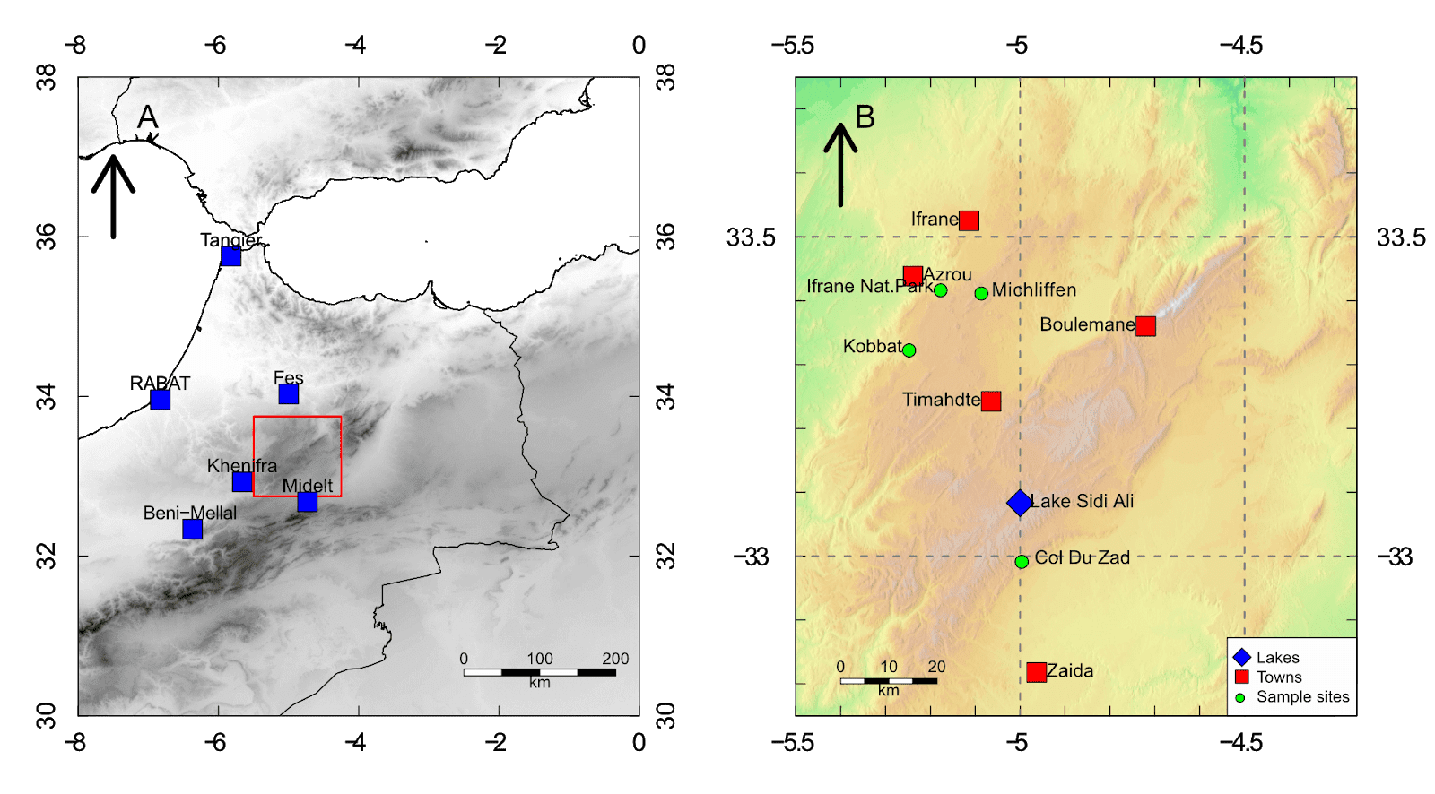
This guide will show you some basic techniques for creating simple, yet effective location maps in R, using freely available data. Stop using screenshots of Google Earth for your location maps, and start making your own! No GIS skills are needed. Read on to see how the create the map below!


Interpolating gridded datasets in R: UV-B data

In my most recent published paper, I analysed the effects of incoming solar UV-B radiation on the geochemistry of Atlas cedar pollen, focused on the Middle Atlas Mountains in Morocco. The study area was relatively small, with sample sites fairly close together.

The UV-B data was obtained from the glUV: Global UV-B radiation dataset, which combines data from NASA's Ozone Monitoring Instrument (OMI) onboard the Aura spacecraft, into grid cells containing average erythemally weighted estimates of daily UV-B radiation. You can read full details of the methods used in the associated research paper (Beckmann et al. 2014) (Available open access).

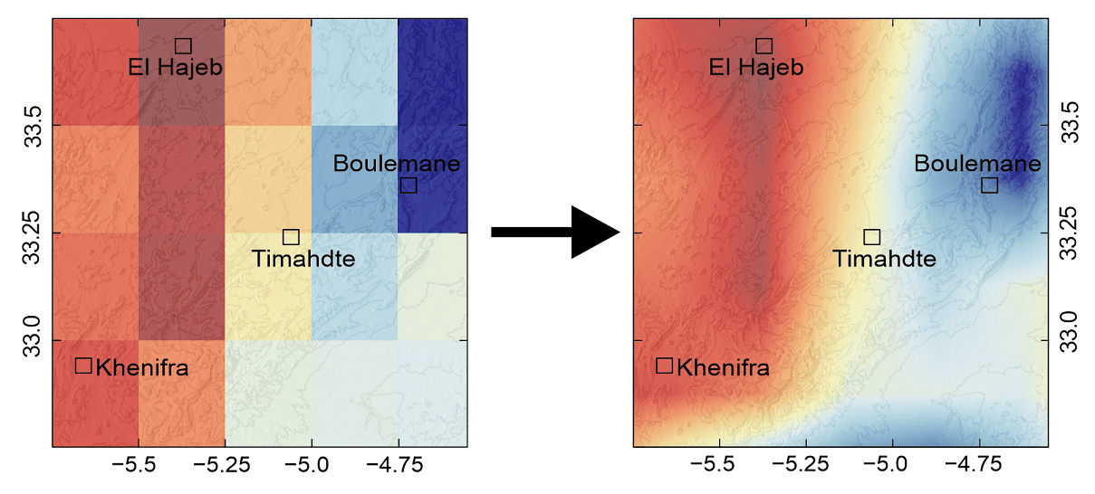
Gridded datasets are an excellent source of data for doing global or macro-scale studies. However, if working in a relatively small area, you may find that your study area is covered by just a few grid cells due to the often low resolution of gridded data. And this can sometimes make it more difficult to carry out analysis.

To overcome the problem, you can interpolate the data to increase the resolution. After interpolation, the gridded data will go from looking like the image on the left, to looking like the image on the right, which is much more detailed for the study area.

Read on to find out how to do this in R!


RasterStacks and raster::plot

Following on from the previous guide looking at WorldClim data, in this guide I take a look at using RasterStacks to import WorldClim datasets. In the previous guide, we used RasterLayers to import the data, so what is the difference? A RasterStack is a collection of RasterLayers bundled together, or stacked into one object. If you're only dealing with a few RasterLayers, then a RasterStack might not be necessary. However, when the number of RasterLayers increase, it can be easier to work with RasterStacks.

For example, if you wanted to look at minimum, maximum, and mean temperature data, along with precipitation data from WorldClim, using RasterLayers would require you to create 48 separate objects. Using a RasterStack, you could instead create 4 objects containing all the data for each variable.

This guide will also take a look at some of the additional options you have when plotting RasterStacks and other raster objects. Did you know that when you plot a raster object in R using plot(), it actually invokes the raster::plot function, while standard objects (e.g. scatterplots) would invoke graphics::plot? The previous guide suggested you might want to plot a figure which includes separate plots for each month of the year, or you might want a minimum and maximum temperature plot? I'll show you how you can do this easily using RasterStacks and raster::plot.


Extracting data and making climate maps using WorldClim datasets

In this guide, i'll show you another way in which you can get climate data, by using WorldClim global climate datasets. This guide will take you through all the steps for downloading, opening, extracting, and plotting the data using R.

I'll show you how you can make some good looking climate maps using WorldClim data, for anywhere in the world. And, the guide will also look at some of the differences between the WorldClim datasets and CRU datasets (we looked at this in earlier guides), and why you might choose to use one or the other.