R has no error bar function? Surely not!
Well, yes and no. Error bars can be added to plots using the arrows() function and changing the arrow head. You can add vertical and horizontal error bars to any plot type. Simply provide the x and y coordinates, and whatever you are using for your error (e.g. standard deviation, standard error).
Read on to see how this is done with examples.
Guide Information
| Title | How to add error bars in R |
| Author | Benjamin Bell |
| Published | April 01, 2019 |
| Last updated | September 30, 2019 |
| R version | 3.5.2 |
| Packages | base |
| Navigation |
This guide has been updated:
- Updates made to improve clarity of this guide, and remove some confusing terminology.
Error bars in R
If you are using base graphics to create your plots, you may have wanted to add error bars to your plot and were left wondering how this is done.
Many people would suggest that R does not have an inbuilt error bar function, while this might *technically* be true, error bars are easily added to any plot using the arrows() function.
Arrows for errors
Lets first first take a look at the arrows() function and how it works. For example, let's draw a vertical and horizontal arrow on a plot:
# Blank plot
x <- 5
y <- 5
plot(x, y, xlim=c(1,10), ylim=c(1,10), axes=FALSE, xlab="x", ylab="y", pch=16, cex=2)
axis(1, 1:10)
axis(2, 1:10)
# Vertical arrow
arrows(x0=x, y0=y-3, x1=x, y1=y+3, code=3, col="blue", lwd=2)
# Horizontal arrow
arrows(x0=x-3, y0=y, x1=x+3, y1=y, code=3, col="red", lwd=2)
Which results in the following:
I have also labelled the start and end point coordinates for each arrow.
Lets take a look at the code to explain how this works.
# Blank plot
x <- 5
y <- 5
plot(x, y, xlim=c(1,10), ylim=c(1,10), axes=FALSE, xlab="x", ylab="y", pch=16, cex=2)
The first part of the code is simple. We have created a plot, plotting the x and y vectors. In this case, both the x and y vectors contain a single element (5). The result is a plot with a single point at x=5 and y=5.
To draw the arrows, we have to tell R the coordinates of the start point (x0 and y0) and the end point (x1 and y1) for the arrow.
Vertical arrows
# Vertical arrow
arrows(x0=x, y0=y-3, x1=x, y1=y+3, code=3, col="blue", lwd=2)
For the vertical arrow, the x0 coordinate is just the x vector (defined earlier as x <- 5). So, on our plot, the arrow will appear at position 5 along the x axis.
The y0 coordinate is the y vector (defined earlier as y <- 5) minus 3. So, 5 - 3 = 2, and therefore our arrow's start position is 2 on the y axis.
The x1 coordinate is also just the x vector, since we want a straight arrow. The y1 coordinate is the y vector, but this time, it is plus 3. So, 5 + 3 = 8, resulting in the arrow's end position being 8 on the y axis.
The start point for the vertical arrow is equivalent to telling R to use x0=5, y0=2, while the end point is equivalent to using x1=5, y1=8.
So why didn't we just R to do that? Because, using plus or minus values in conjunction with the position of the point is necessary for correctly plotting error bars.
Horizontal arrows
# Horizontal arrow
arrows(x0=x-3, y0=y, x1=x+3, y1=y, code=3, col="red", lwd=2)
For the horizontal arrow, the x0 coordinate is the x vector (defined earlier as x <- 5) minus 3. The y0 coordinate is just the y vector (defined earlier as y <- 5).
The x1 coordinate is the x vector, but this time, it is plus 3. The y1 coordinate is also just the y vector since we want a straight arrow.
So, the start point for the vertical arrow is equivalent to telling R to use x0=2, y0=5, while the end point is equivalent to using x1=8, y1=5.
Turning arrows into error bars
So now you understand how to draw arrows, but how do you turn them into error bars?
Simple, we just add two more arguments to the arrows() function:
# Vertical arrow
arrows(x0=x, y0=y-3, x1=x, y1=y+3, code=3, angle=90, length=0.5, col="blue", lwd=2)
# Horizontal arrow
arrows(x0=x-3, y0=y, x1=x+3, y1=y, code=3, angle=90, length=0.5, col="red", lwd=2)
angle=90 tells R to draw the arrow heads as straight lines, and length=0.5 tells R how long to make the error bars.
Now you have error bars!
Error bar examples
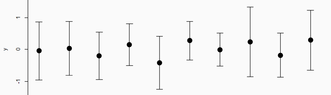
The examples above show how error bars are drawn in R. Here's a "real world" example of how you might use the standard deviation for the error bars on a scatter plot:
# Generate random data
set.seed(100)
m <- matrix(rnorm(100), ncol=10)
y <- apply(m, 2, mean) # Calculate mean
y.sd <- apply(m, 2, sd) # Calculate standard deviation
x <- 1:10
# Plot
plot(x, y, ylim=c(-3, 3), xlab="x", ylab="y", pch=16, cex=2)
# Add error bars
arrows(x0=x, y0=y-y.sd, x1=x, y1=y+y.sd, code=3, angle=90, length=0.1)
In this example, we calculate the mean values from our random dataset, and the standard deviation; the y.sd object.
We can take a look at these in the R console:
> y
 [1] -0.017957164  0.233691459 -0.129142366  0.314116572  0.006836221 -0.043229727  0.196632374
 [8] -0.406163801  0.077907762 -0.203565705
> y.sd
 [1] 0.5611186 0.8602353 0.6753273 0.7416699 1.1994489 1.5223430 0.9118494 1.2728778 1.0812995
[10] 1.2457779
For the error bars, rather than using the same plus or minus value for coordinates of the error bar, we use the standard deviation value for each data point, which we take from the y.sd object: y0=y-y.sd and y1=y+y.sd.
This results in the following plot:
If you wanted to add error bars to a bar plot, the x value becomes the barplot "midpoint", which can be calculated simply by creating the barplot as an object:
# Random data
set.seed(100)
m <- matrix(runif(1000, min=1, max=10), ncol=10)
y <- apply(m, 2, mean)
y.sd <- apply(m, 2, sd)

# Calculate midpoints
mid <- barplot(y)

# Plot barplot
barplot(y, ylim=c(0, 10), col=rainbow(10))
# Add error bars
arrows(x0=mid, y0=y-y.sd, x1=mid, y1=y+y.sd, code=3, angle=90, length=0.1)
For the error bars, the x0 and x1 values are now the midpoints of the barplot, while the y0 and y1 values remain as the standard deviation.
You can see the midpoint values in the R console:
> mid
      [,1]
 [1,]  0.7
 [2,]  1.9
 [3,]  3.1
 [4,]  4.3
 [5,]  5.5
 [6,]  6.7
 [7,]  7.9
 [8,]  9.1
 [9,] 10.3
[10,] 11.5
And the resulting bar plot will look like this:
And that's how you can add error bars to plots created with base graphics. Thanks for reading, please leave any comments or questions below.
Further reading
A quick guide to pch symbols - A quick guide to the different pch symbols which are available in R, and how to use them. [R Graphics]
A quick guide to line types (lty) - A quick guide to the different line types available in R, and how to use them. [R Graphics]
Thank you so much such easy to understand explanation.
ReplyDeletegreat tutorial!
ReplyDeleteFantastic:)
ReplyDelete