In my previous guide, I showed you how to download and extract precipitation and temperature climate data from CRU datasets. Now that you have the raw data - i'll guide you through some of the ways in which you can work with, and manipulate this data.
From grouping your sample sites, to calculating annual data or seasonal data, to defining a climate period and then calculating changes to conditions since this period to observe climate change trends. I'll also show you how to plot the data to create climate graphs for your sites.
Guide Information
| Title | Working with extracted CRU climate data |
| Author | Benjamin Bell |
| Published | January 18, 2018 |
| Last updated | August 17, 2021 |
| R version | 3.4.2 |
| Packages | base; raster; ncdf4; gdata |
| Navigation |
This guide has been updated:
- Since this guide was originally published, CRU have released new versions of the CRU TS dataset. You can still download the older versions of the dataset, or you can download the latest version and follow this guide using the latest data. The code will still work, but you will need to update parts (e.g. the years) to reflect the newer dataset.
This is a 4 part guide:
| Part 1: Getting Climate Data | Downloading CRU climate data and opening it in R. |
| Part 2: Working with extracted CRU climate data | How to use the downloaded climate data, from calculating trends to plotting the data. |
| Part 3: Extracting data and making climate maps using WorldClim datasets | How to obtain WorldClim climate data, importing it into R, and how to calculate trends and plot climate maps. |
| Part 4: RasterStacks and raster::plot | An update to part 3, this guide shows you an easier way to import WorldClim data into R by using RasterStacks. |
Working with and manipulating CRU climate data
This is part two of a guide series for downloading, extracting and working with climate data. If you missed part one, you can find that here, which guides you through the process of getting CRU climate data. You'll need this data to follow this guide.
In the previous guide we extracted precipitation and temperature data for four sites in the UK, and we exported this to two spreadsheets named "Precipitation Data.csv" and "Temperature Data.csv".
Rather than repeat the steps for extracting the data, lets simply import the spreadsheets back into R. If you do not have these spreadsheets, you can download them for use in this guide from Google Docs: Precipitation Data and Temperature Data
# Import extracted climate data
precip <- read.csv("Precipitation Data.csv", header=TRUE, row.names=1, sep=",", check.names=FALSE) # Precipitation
temp <- read.csv("Temperature Data.csv", header=TRUE, row.names=1, sep=",", check.names=FALSE) # Mean monthly temperature
You'll notice a couple of differences in this import command to what we used in the last guide.
Firstly, the row.names argument simply states "1" rather than the name of the column. This is useful when the column name is missing, as "1" tells R that the first column in the spreadsheet should be row names.
Secondly, there is a new argument check.names=FALSE - Since the column names in the imported spreadsheet start with a number, if you import the spreadsheet without this argument, the column names in R would be prefixed with an "X". This argument keeps the names exactly how they are formatted in the spreadsheet.
Now that we have the raw climate data loaded into R, there are several things we can do. For example, you might want to calculate annual precipitation levels, or calculate mean annual temperatures. You might also want to look at trends in the data, such as the average climate conditions for each decade or season, and plot these changes. All of these things are really simple to perform using R!
Grouping sample sites
In this example we are working with only four sites - but for your own project you might be working with much more then this, and you might want to group some of the sites together, for example, to get average climate conditions for a larger geographical area.
Using the example data, lets create two groups: "North" and "South", and calculate the average conditions using "Manchester" and "Liverpool" data for the "North" group, and "Oxford" and "London" data for the "South" group. We'll add this data to our existing data frames (precip and temp), which we created when we imported the climate data.
# Group samples sites, and calculate average data
# Precipitation
precip <- rbind(precip, North=colMeans(precip[1:2,])) # "North" group
precip <- rbind(precip, South=colMeans(precip[3:4,])) # "South" group
In the above code, we have told R that we want to create a new row and combine it with our existing data frame object "precip", using the rbind() command. The first argument of rbind() tells R which object we want to add the new row to. The second argument, "North" becomes the name of the new row. Finally, the command following "=" tells R what data to assign to the new row ("North").
In the first instance, we want to know the average data for Manchester and Liverpool. The command colMeans() will calculate the mean (average) values for every column in a data frame object. However, we only want to know the mean values for our groups, so we must also specify which rows to use when calculating the column means, by subsetting the data.
R is very powerful when it comes to subsetting data (i.e. selecting only the data you want). You subset data from an object using square brackets, e.g. precip[] For more details on subsetting data, have a look at this guide from Quick-R to get started.
Back to our example, colMeans(precip[1:2,]) tells R to calculate mean values for every column using the first two rows of our data frame "precip", while colMeans(precip[3:4,]) tells R to calculate mean values for every column using the third and fourth rows.
If you wanted to know the mean column values for every row, you would simply use colMeans(precip)
If you were to now look at the "precip" data frame using: fix(precip) it should now contain two additional rows with mean data representing sites in the north and south.

You should repeat these steps for the temperature data, using the same code, but replacing "precip" with "temp". It is advisable to calculate your "groups" first, before further analysis.
Calculating annual climate data
Update: If you are using a later version of the CRU TS dataset, you need to update the code below to reflect the additional period of time that is available. e.g. years <- 1901:2020
The extracted data from CRU provides monthly climate data for each month between 1901 to 2016. But you might want to know what the annual values are, and this is easy to calculate in R. For precipitation, we want to know the total annual precipitation for each year, while for temperature, we want to know the mean annual temperature.
Starting with the precipitation data, we'll use the following code to create a new data frame object that contains total annual precipitation values.
years <- 1901:2016
precip.year.total <- as.data.frame(sapply(years, function(x) rowSums(precip[, grep(x, names(precip))])))
names(precip.year.total) <- years # Rename columns in the new data frame object
To calculate the annual data, we have to use several commands, and at first glance, the code looks confusing.
To explain whats happening, lets break down the code into smaller chunks. The first line of code creates a vector object named "years" which contains the years between 1901 to 2016. (Type "years" in to the R console to see)
> years
  [1] 1901 1902 1903 1904 1905 1906 1907 1908 1909 1910 1911 1912 1913 1914 1915
 [16] 1916 1917 1918 1919 1920 1921 1922 1923 1924 1925 1926 1927 1928 1929 1930
 [31] 1931 1932 1933 1934 1935 1936 1937 1938 1939 1940 1941 1942 1943 1944 1945
 [46] 1946 1947 1948 1949 1950 1951 1952 1953 1954 1955 1956 1957 1958 1959 1960
 [61] 1961 1962 1963 1964 1965 1966 1967 1968 1969 1970 1971 1972 1973 1974 1975
 [76] 1976 1977 1978 1979 1980 1981 1982 1983 1984 1985 1986 1987 1988 1989 1990
 [91] 1991 1992 1993 1994 1995 1996 1997 1998 1999 2000 2001 2002 2003 2004 2005
[106] 2006 2007 2008 2009 2010 2011 2012 2013 2014 2015 2016
The second line of code creates the new data. Firstly, precip.year.total <- as.data.frame(...) tells R that we want to create a new data frame object called "precip.year.total". In order to calculate the yearly data automatically, we use the sapply(...) command to apply a function(x) to the "precip" data frame.
The function(x) we create, tells R we want to calculate the total value of each row in the "precip" data frame using rowSums(), but since we want to know the total value for each year rather than the entire row (which would be 116 years of data!), we need to subset the data by using grep() to pattern match the years (contained in the "years" vector object).
grep(x, names(precip))]) will match the column names in the "precip" data frame names(precip) to "x", and in this example, "x" is the vector object "years".
The third line of code renames the columns in the "precip.year.total" data frame to the values in the "years" object, otherwise they would be named "V1", "V2" etc.
The new dataframe should look something like this:

If you are still confused, have a play around with the code, changing different variables to see what happens, which should make things clearer.
For example, instead of calculating total annual precipitation, you could calculate the total precipitation of each month for the period 1901 to 2016:
# Calculate Total monthly rainfall between 1901 and 2016.
month <- c("Jan", "Feb", "Mar", "Apr", "May", "Jun", "Jul", "Aug", "Sep", "Oct", "Nov", "Dec")
precip.month.total <- as.data.frame(sapply(month, function(x) rowSums(precip[, grep(x, names(precip))])))
names(precip.month.total) <- month # Rename columns in the new data frame object
Which should look something like this:

But, it doesn't really make much sense to do this, so instead, you could calculate the mean monthly precipitation for each month for the period 1901 to 2016, by using rowMeans() instead of rowSums() e.g.
# Calculate mean monthly rainfall between 1901 and 2016.
precip.month.mean <- as.data.frame(sapply(month, function(x) rowMeans(precip[, grep(x, names(precip))])))
names(precip.month.mean) <- month # Rename columns in the new data frame object
Which should look something like this:

For the temperature data, you would want to calculate mean annual temperature, so again, you would use rowMeans() instead of rowSums() in your code.
# Calculate mean annual temperature values
temp.year.mean <- as.data.frame(sapply(years, function(x) rowMeans(temp[, grep(x, names(temp))])))
names(temp.year.mean) <- years # Rename columns in the new data frame object
Which should look something like this:

Calculating climate data for each decade, or defined period
In the previous example we created yearly data, but, what if we wanted to look at the average climate data for each decade, or longer. Technically, climate refers to weather data over a long period of time, usually 30 years. There are several ways in which you could calculate this, but it would depend on whether you wanted to look at monthly or yearly data.
Annual data
We'll start by looking at Mean Annual Precipitation (MAP) for each decade in our data. We'll create a new data frame object, and calculate MAP using the yearly data:
# Calculate mean annual precipitation (MAP) for each decade
dec <- list(1:9, 10:19, 20:29, 30:39, 40:49, 50:59, 60:69, 70:79, 80:89, 90:99, 100:109, 110:116)
precip.decade.map <- as.data.frame(sapply(dec, function(x) rowMeans(precip.year.total[, x])))
There are two parts of code needed to create the decadal data. Firstly, we need to create a list() object where we will group the column numbers of each decade from the "precip.year.total" data frame. e.g. columns 1 through 9 contain data for the period 1901 to 1909.
The benefits of creating a list, is that you can have total control on the groups. As the CRU data starts from 1901, it means the first decade has 9 years rather than 10. And since the data ends in 2016, it means the final decade contains only 7 years of data. You can check how many columns are grouped together in the list by using the lengths() command, while length() will tell you the total number of groups. e.g.
> lengths(dec)
 [1]  9 10 10 10 10 10 10 10 10 10 10  7
> length(dec)
 [1] 12
The second part of the code is similar to what we used in the previous examples. However, rather than subsetting the data using grep(), we simply use the "dec" list object.
Lets rename the columns to something useful, such as the start of each decade. Rather than type out each decade manually, lets create a sequence seq() of numbers:
# Rename columns using a sequence
dec.n <- seq(from=1900, to=2010, by=10)
names(precip.decade.map) <- dec.n
This code should be pretty self-explanatory! and the resulting data frame should look something like this:

You can calculate mean annual temperatures in the same way, but remember to change the names.
# Calculate mean annual temperatures for each decade
temp.decade.mean <- as.data.frame(sapply(dec, function(x) rowMeans(temp.year.mean[, x])))
names(temp.decade.mean) <- dec.n
It is often easier to understand data and observe trends by visualising the data. Lets create a simple plot showing precipitation, and a seperate plot showing temperature for Manchester.
# Simple plot showing precipiation and temperature for each decade
layout(matrix(1:2, ncol=2))
plot(dec.n, precip.decade.map[1,], type="o", col="blue")
plot(dec.n, temp.decade.mean[1,], type="o", col="red")
Here, layout() and matrix() tell R to create a plot window that will contain two plots side by side. Next we use plot() to plot our data. Since the data is in a data frame object and we want to plot a row, we first define the x axis as "dec.n" - because this object contains our decades, then the y axis as precip.decade.map[1,], which tells R to use the data in row 1 of the precip.decade.map data frame, which contains Manchester data.
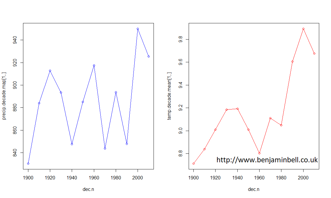
From these plots, it is easy to see that while precipitation has been quite variable during the last ~100 or so years in Manchester, temperature has steadily increased.
There is a better way to look at climate trends however. Instead of looking at the average climate data for each decade, lets average the climate data over a 30 year period between 1970 and 2000. This will be used as our baseline climate conditions.
# Average climate between 1970 and 2000
precip.base.map <- rowMeans(precip.year.total[70:99])
temp.base.mean <- rowMeans(temp.year.mean[70:99])
Using this data as a baseline, we can now calculate annual changes to climate, which can often make it easier to understand climate trends.
# Calculate change in climate using 1970 to 2000 data as a baseline
precip.change <- precip.year.total - precip.base.map
temp.change <- temp.year.mean - temp.base.mean
Or, you could also calculate the change as a percentage:
# Calculate change as a percentage
precip.pc <- precip.year.total / precip.base.map - 1
precip.pc <- precip.pc * 100
temp.pc <- temp.year.mean / temp.base.mean - 1
temp.pc <- temp.pc * 100
Now we can plot annual changes in climate using the average climate conditions between 1970 and 2000 as the baseline. However, we first need to convert our data. Strictly speaking, climate observations are timeseries data, so we need to create a timeseries ts() object from our data.
Since the data we want to use is stored in a row of a data frame, we need to first convert it to a numeric vector using the as.numeric() command. Then we can create the ts() object. In the timeseries object, the start argument is used to specify the start date, while the frequency=1 argument tells R that this timeseries contains annual data.
You can then plot the data, and use abline(h=0) to add a baseline indicator to the figure.
# Convert Precipitation data for Manchester to time series and plot data
precip.man <- as.numeric(precip.change[1,]) # First convert to numeric vector
precip.man <- ts(precip.man, start=1901, frequency=1) # Then convert to timeseries object
plot(precip.man, col="blue")
abline(h=0)
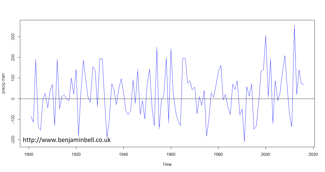
And, you can repeat these steps to also plot changes in mean annual temperature.
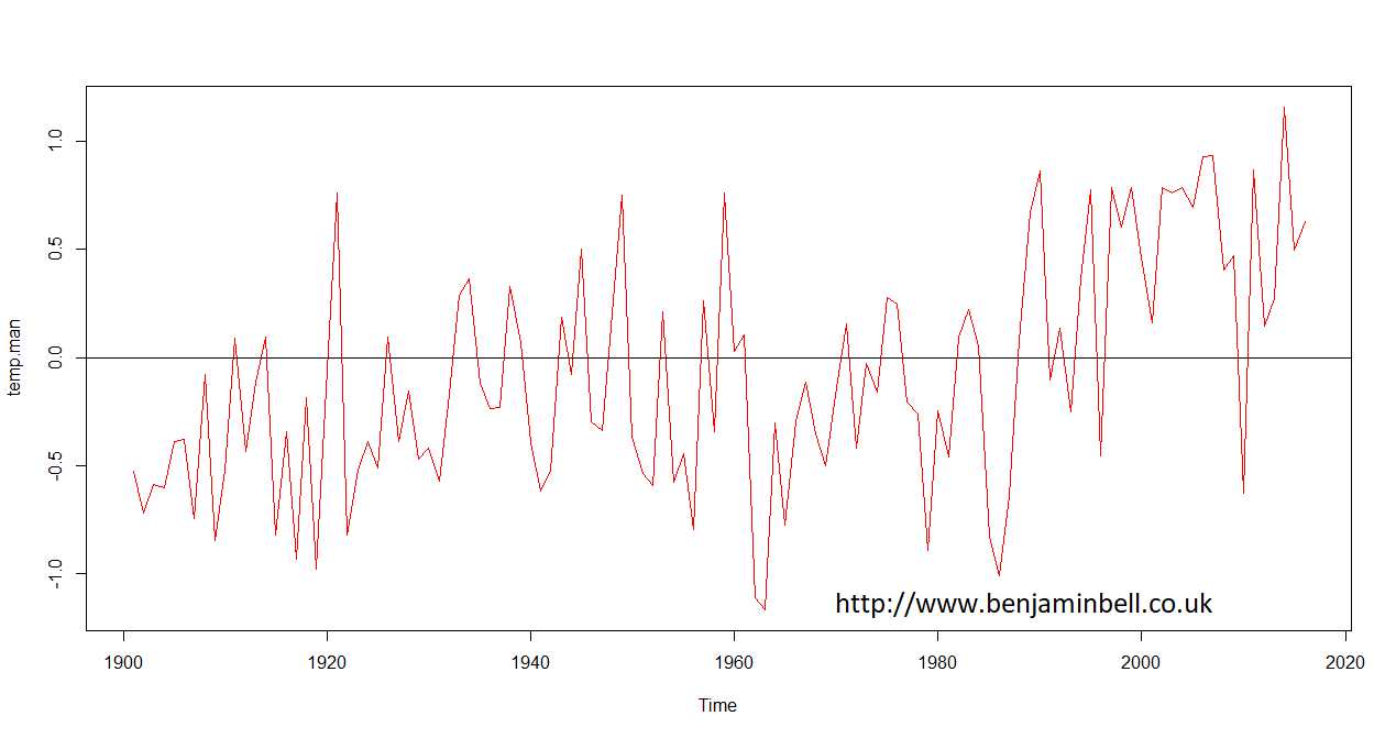
Timeseries are powerful objects in R which allow you to do things such as forecasting and modelling data. I'll come back to using timeseries objects in a future guide.
Monthly data
To look at the average monthly data, we'll calculate this from the original CRU data frames containing monthly climate data between 1901 and 2016. For this example, we'll create average monthly data for the period between 1970 and 2000.
First, we'll create a new data frame object with only the data we want by subsetting the larger data frames (precip and temp). So, we need to know what the column number range is, for the period of time we want data for, which we can get by using the which() command in the R console:
> which(colnames(precip)=="1970_Jan")
 [1] 829
> which(colnames(precip)=="1999_Dec")
 [1] 1188
So we can now go ahead and subset our data using these values:
precip1970 <- precip[829:1188]
temp1970 <- temp[829:1188]
If you wanted to check the new data frames contain the correct data, simply type the object name in to the R console. Alternatively, you could use length(precip1970), which will return a value of 360, and 360 / 12 = 30 years.
To calculate mean monthly values for this period, we'll again use grep() to subset our data.
# Calculate mean monthly data
month <- c("Jan", "Feb", "Mar", "Apr", "May", "Jun", "Jul", "Aug", "Sep", "Oct", "Nov", "Dec")
precip1970.mean <- as.data.frame(sapply(month, function(x) rowMeans(precip1970[, grep(x, names(precip1970))])))
names(precip1970.mean) <- month # Rename columns in the new data frame object
Which should look like this:

Now, you can repeat this for the temperature data.
# Calculate mean monthly data
temp1970.mean <- as.data.frame(sapply(month, function(x) rowMeans(temp1970[, grep(x, names(temp1970))])))
names(temp1970.mean) <- month # Rename columns in the new data frame object

You could modify this code to define any period of time you like, and also modify the previous example code to calculate and plot monthly changes in climate from this baseline.
And now that you have average monthly climate conditions, lets create a nice plot to show them off!
# Precipitation and Temperature climate graph for Manchester
# Full guide available at http://www.benjaminbell.co.uk

# Convert data to numeric vector
precip1970.man <- as.numeric(precip1970.mean[1,])
temp1970.man <- as.numeric(temp1970.mean[1,])

# Get midpoint positions of barplot x axis
mid <- barplot(precip1970.man, xlim=c(0, 14.5))

# Plot a barplot with precipitation data
par(mar=c(5,5,5,5)) # Set the plot margins
barplot(precip1970.man, beside=TRUE, ylim=c(0, 100), xlim=c(0, 14.5), ylab="Mean Precipitation (mm)", names.arg=month, las=1, col="deepskyblue")

# Plot temperature graph on top of precipitation graph
par(new=TRUE)
plot(mid, temp1970.man, type="o", lwd=3, ylim=c(0, 30), xlim=c(0, 14.5), axes=FALSE, ann=FALSE, col="red")

# Plot axis to the right side and label
axis(4, las=2, tck=-0.02)
mtext("Temperature (C)", side=4, line=3)
title(main="Average Manchester Climate\n1970 to 2000")

# Draw a box around the plot
box()
Which will result in the following plot. I'll leave you to figure out the code :) (Hint, try ?plot in the R console for help).

Calculating seasonal climate data
For the final part of this guide, we'll have a look at creating seasonal data. So far, we have used two different methods for subsetting data, and for the seasonal data i am going to show you another method!
In this example, we are going to create seperate data frames for each season, which will contain the seasonal data for each year. We'll start by defining the seasons - we'll set up winter later:
spring <- c("Mar", "Apr", "May")
summer <- c("Jun", "Jul", "Aug")
autumn <- c("Sep", "Oct", "Nov")
In order to subset our data this time, we are going to use the "gdata" package. Use install.packages("gdata") to install, if you do not already have this package installed.
Now that the seasons are set up, we'll use the matchcols() command from the gdata package to easily select the columns we want from the precip data frame.
library("gdata")
# Get spring column names
spring.mc <- matchcols(precip, with=spring, method="or")
In the above code, precip is the data frame object we will use to get the column names from. You could use either the precip or temp data frame here, since the column names are the same in both. with=spring is the vector object that contains the names of the spring months, and method="or" tells R to select all columns matching either "Mar" or "Apr" or "May".
If you type "spring.mc" into the R console, you should get a matrix containing all the column names from the "precip" data frame that matches with the variables in the "spring" vector object.
> spring.mc
       Mar        Apr        May
  [1,] "1901_Mar" "1901_Apr" "1901_May"
  [2,] "1902_Mar" "1902_Apr" "1902_May"
  [3,] "1903_Mar" "1903_Apr" "1903_May"
  [4,] "1904_Mar" "1904_Apr" "1904_May"
  ...
Next, we'll create two new data frames which will only contain climate data for the spring months.
# Create spring climate data frames
precip.spring <- subset(precip, select=spring.mc) # Precipitation
temp.spring <- subset(temp, select=spring.mc) # Temperature
Which will result in the following data frame. Notice the column order: 1901_Mar, 1902_Mar, 1903_Mar etc. which is not really that useful, but the data frame does now contain only spring data.

Next, we'll subset the data again to create annual data. Remember, for precipitation we are interested in the total precipitation for the season, while for temperature data, we are interested in the mean temperature for the season. This uses the same commands we previously used to create yearly data earlier in this guide.
# Create yearly seasonal data
years <- 1901:2016
precip.spring.year <- as.data.frame(sapply(years, function(x) rowSums(precip.spring[, grep(x, names(precip.spring))])))
names(precip.spring.year) <- years # Rename columns in the new data frame object
Which will result in the following data frame showing total spring precipitation for each year.

The following code will create average spring temperatures for each year:
temp.spring.year <- as.data.frame(sapply(years, function(x) rowMeans(temp.spring[, grep(x, names(temp.spring))])))
names(temp.spring.year) <- years # Rename columns in the new data frame object
Using this code, you can also create seasonal data for the summer and autumn (fall).
To create the winter seasonal data, we need to take some additional steps. This is because the code works by matching the months of the season to the year. However, winter includes two different years, e.g. 1901_Dec, 1902_Jan and 1902_Feb.
There is a simple work around, which involves offsetting the year by +1 for December. e.g. 1901_Dec would become 1902_Dec. So when you run the command to subset the data, it will match the "correct" December with January and February data. Let's do this for winter precipitation:
# Create winter data
winter <- c("Dec", "Jan", "Feb")
winter.mc <- matchcols(precip, with=winter, method="or")
precip.winter.x <- subset(precip, select=winter.mc) # Precipitation
The first part of the code is the same as for the other seasons. Next, we'll create a new data frame containing just the December months, and we'll offset the years by 1.
# Subset december data
precip.winter.off <- precip.winter.x[,1:116]

# Offset the years
year.off <- 1902:2017
names(precip.winter.off) <- paste(rep(year.off, each=1), rep("Dec", times=116), sep="_")
Next, we'll recombine the offset December data with the original Jan and Feb data. Note, that we'll remove the "2017_Dec" column when we recombine the data.
# Recombine the offset December data with Jan and Feb
precip.winter <- cbind(precip.winter.off[,1:115], precip.winter.x[117:348])
Now, you can run the same code to create the yearly seasonal data as you did previously.
# Create yearly winter data.
precip.winter.year <- as.data.frame(sapply(years, function(x) rowSums(precip.winter[, grep(x, names(precip.winter))])))
names(precip.winter.year) <- years # Rename columns in the new data frame object
You can follow those steps to also create mean winter temperature data.
And thats it! Thanks for reading this guide, please leave any comments or questions below
This is a 4 part guide:
| Part 1: Getting Climate Data | Downloading CRU climate data and opening it in R. |
| Part 2: Working with extracted CRU climate data | How to use the downloaded climate data, from calculating trends to plotting the data. |
| Part 3: Extracting data and making climate maps using WorldClim datasets | How to obtain WorldClim climate data, importing it into R, and how to calculate trends and plot climate maps. |
| Part 4: RasterStacks and raster::plot | An update to part 3, this guide shows you an easier way to import WorldClim data into R by using RasterStacks. |
Further reading
Extracting CRU climate data - Part 1 of this guide.
Extracting Worldclim climate data - Part 3 of this guide!
Cheers Ben, this post helped saved me a ton of time in extracting climate data.
ReplyDeleteOne quick question, when given the below, any thoughts on how to extract standard deviations for each month across years, rather than means? Something like using apply rather than sapply? Any help would be mega appreciated, best, Tom.
# Calculate mean monthly rainfall between 1901 and 2016.
precip.month.mean <- as.data.frame(sapply(month, function(x) rowMeans(precip[, grep(x, names(precip))])))
names(precip.month.mean) <- month # Rename columns in the new data frame object
Hi Tom, apologies for the long delay in replying!
DeleteYou are correct, you need to use apply to get the standard deviations.
Here's an example where standard deviations are calculated for the month of January (based on the code in this guide):
# Load gdata
library("gdata")
# Use matchcols to select column names with January
jan <- matchcols(precip, with="Jan", method="or")
# Create new data frame with just the jan data
precip.jan <- subset(precip, select=jan)
# Apply sd to rows
jan.sd <- apply(precip.jan, 1, sd)
This would calculate sd for all the years in the dataset. You could change which years the standard deviation is calculated for by subsetting the data again:
# Standard deviation for 1901 to 1910
jan.sd.1910 <- apply(precip.jan[1:10], 1, sd)
Hope this helps!
Hi Ben,
ReplyDeleteThank you for this great tutorial.
I have a question. What does the value "117:348" represent in this line below:
# Recombine the offset December data with Jan and Feb
precip.winter <- cbind(precip.winter.off[,1:115], precip.winter.x[117:348])
It represents the months of January and February.
DeleteTake a look at the data in R to see using: fix(precip.winter.x)
Best wishes,
Ben
Thank you SO much for this tutorial!
ReplyDeleteIt is a great tutorial. I am using your codes to analyze climate data of my country Bhutan. I also have interest to downscale climate for Bhutan and develop a high resolution data. Could you also post your codes on this? Thanks a lot.
ReplyDelete> pre <- brick("D:\\Rstudio\\climate data\\cru_ts3.26.1901.2017.pre.dat.nc"), varname = "pre"
ReplyDeleteError: unexpected ',' in "pre <- brick("D:\\Rstudio\\climate data\\cru_ts3.26.1901.2017.pre.dat.nc"),"
> pre <- brick("D:\\Rstudio\\climate data\\cru_ts3.26.1901.2017.pre.dat.nc")
Error in R_nc4_open: Permission denied
Error in ncdf4::nc_open(filename, readunlim = FALSE, suppress_dimvals = TRUE) :
Error in nc_open trying to open file D:\Rstudio\climate data\cru_ts3.26.1901.2017.pre.dat.nc (return_on_error= FALSE )
> pre <- brick("D:\\Rstudio\\climate data\\cru_ts3.26.1901.2017.pre.dat.nc"), varname = "pre"
Error: unexpected ',' in "pre <- brick("D:\\Rstudio\\climate data\\cru_ts3.26.1901.2017.pre.dat.nc"),". I could not access CRU TS data. Could you help me find the solution to access data?
Hi Dahal,
DeleteFor this line of code:
pre <- brick("D:\\Rstudio\\climate data\\cru_ts3.26.1901.2017.pre.dat.nc"), varname = "pre"
It should be written as follows:
pre <- brick("D:\\Rstudio\\climate data\\cru_ts3.26.1901.2017.pre.dat.nc", varname = "pre")
The closing bracket was in the wrong place.
For the other error - please check the file and folder locations are correct, and that all names are typed exactly, remembering that R is case sensitive.
One way to check file/folder names in R is to use the list.files() function - for example:
list.files("D:\\Rstudio\\climate data")
If that results in an error - then you either have a typo, or there is a file permission problem which relates to your system configuration, and unfortunately, I cannot help there :)
Best wishes,
Ben