Bathymetric maps are topographic maps of water bodies (oceans, seas, lakes, rivers), equivalent to Digital Elevation Models (DEMs), except for submerged terrain.
Useful in their own right, bathymetric maps can also improve the look of maps created using DEMs, giving depth to water features.
This 2-part guide shows you how to create bathymetric maps in R using freely available data from online sources, how to import and plot this in R. Part 2 explores using different colour schemes/palettes for really effective maps. Read on for more!

Guide Information
| Title | Bathymetric maps in R: Getting and plotting data |
| Author | Benjamin Bell |
| Published | August 22, 2019 |
| Last updated | |
| R version | 3.6.1 |
| Packages | base; raster |
| Navigation |
This is a 2 part guide:
| Part 1: Getting and plotting data | How to create bathymetric maps in R using freely available data from online sources. |
| Part 2: Colour palettes and break points | How to create effective colour schemes using break points, which is useful for when plotting bathymetric maps. |
Overview
Bathymetric maps (or charts) are the equivalent to Digital Elevation Models (DEMs) for submerged terrain. They provide topographic data for water bodies including; oceans, lakes and rivers.
In the previous guide (DEMs and where to find them), I looked at creating maps using different DEMs in R. However, these maps do not show any topographic information for water bodies. So, if for example you were interested in creating a map of the coast of Portugal, a DEM would only show you the land topography.
This guide will take a look at two sources of global bathymetric data (ETOPO1 and GEBCO 2019). Both of these datasets show the topography of the worlds oceans and seas, which they combine with a DEM so that you can create maps of the land and sea. There is of course loads of other bathymetric data available, which I'll also cover, although the list is not exhaustive.
ETOPO1
ETOPO1 (doi: 10.7289/V5C8276M) is a global relief model which integrates both bathymetric data and a DEM at 1 arc-minute resolution.
The bathymetric data is based on numerous sources, while the land topography is largely based on SRTM data. More information is available in the ETOPO1 documentation.
Two versions of the model are available. The "bedrock" version depicts the elevation of bedrock under the Antarctic and Greenland ice sheets, whereas the "ice surface" version shows the elevation of these ice sheets (and not the underlying bedrock).
ETOPO1 Bedrock
| Horizontal datum | WGS84 |
| Vertical datum | Sea level |
| Spatial resolution | ~2 kilometres (1 arc-minute) |
| Format | GeoTiff, netCDF |
| Raster size | Whole world or custom grid |
| Download | NOAA |
The ETOPO1 Bedrock data can be downloaded as a global file as a GeoTiff, or in netCDF format from NOAA. There is a "grid-registered" and "cell-registered" version, with the grid-registered version being the authoritative version. Download this version if you are not sure which to use.
Alternatively, you can use the grid extract tool to download the data for which ever area you specify.
ETOPO1 Ice surface
| Horizontal datum | WGS84 |
| Vertical datum | Sea level |
| Spatial resolution | ~2 kilometres (1 arc-minute) |
| Format | GeoTiff, netCDF |
| Raster size | Whole world or custom grid |
| Download | NOAA |
The ETOPO1 Ice surface data can also be downloaded as a global file as a GeoTiff, or in netCDF format from NOAA. Like the bedrock version, there is a "grid-registered" and "cell-registered" version for the ice surface data, with the grid-registered version being the authoritative version. Download this version if you are not sure which to use.
Alternatively, you can use the grid extract tool to download the data for which ever area you specify.
If you use the grid extract tool, you will be presented with a screen that looks like this:

To download a specific area, click the first icon in the top right corner ("Select with rectangle"), and draw an area on the map. Then using the options at the bottom, select the layer, the output format, and click the download data link. Alternatively, you can input specific grid coordinates using the second icon ("Select with coordinates").

To load the data in R, first set the working directory to where you have saved the bathymetric file (for example "/R/maps/bathymetry/"). We'll use the raster package to load the file, and for this example, we'll use the global ETOPO1 data:
# Load raster package
library(raster)
# Load ETOPO1 data
etopo.b <- raster("ETOPO1_Bed_g_geotiff.tif")
etopo.i <- raster("ETOPO1_Ice_g_geotiff.tif")
If you downloaded a specific area using the grid extract tool, change the file name in the above code. To plot the data, simply use plot(), for example:
# Plot ETOPO1 bedrock
plot(etopo.b)
# Plot ETOPO1 Ice surface
plot(etopo.i)
Compare the bedrock version:
And the ice surface version:
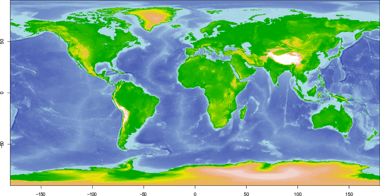
Please note, using the default plot() options in R, your plot will look different to the above images. I have altered the colour scheme, to see how this is done, check out the part 2 of this guide.
GEBCO_2019
| Horizontal datum | WGS84 |
| Vertical datum | Sea level (some shallow water areas use a different datum) |
| Spatial resolution | ~500 metres (15 arc-seconds) |
| Format | netCDF, GeoTiff, ESRI ASCII |
| Raster size | Whole world or custom grid |
| Download | GEBCO (Registration required to download custom grid) |
GEBCO_2019 or General Bathymetric Chart of the Oceans, is a global terrain model integrating bathymetric data and a DEM at 15 arc-seconds resolution. The 2019 grid is an update over the previous 2014 grid offering improved resolution. This data is part of the "Seabed 2030" project to map 100% of the world's oceans.
The gridded ocean and land topography data is built upon SRTM15_Plus data. Then, multibeam bathymetric data is used for areas where it is available to improve the dataset. More information is available in the GEBCO documentation.
You can download the entire grid from the GEBCO webpage. It is available in netCDF format, and is a ~12 gigabyte download. You can also download the source identification grid which details the data source for each grid cell.
If you prefer, you can download a user-defined area rather than the entire grid. You should select the area on the map, choose the data format, and then click "Add data to basket". Clicking "View basket" will then take you to the British Oceanographic Data Centre website where you will need to register in order to download the data.
To load the data in R, we will use the raster package and ncdf4 package. Set the working directory to where you have downloaded the data, and then use the following code:
# Load packages
library(ncdf4)
library(raster)
# Load GEBCO_2019
gebco <- raster("GEBCO_2019.nc")
If you downloaded a user-defined grid, you should change the file name to the name of that data.
With netCDF files, the data contained within is self-describing, so you can examine this to understand the dataset. Type the following code in to the R console to see more details about the netCDF file:
nc_open("GEBCO_2019.nc")
To plot the data, simply use plot(), for example:
# Plot GEBCO_2019
plot(gebco)

At the global scale, there appears to be no difference between the GEBCO_2019 data and the ETOPO1 data. So, lets take a closer look at the coast of Portugal comparing the two datasets:

It's still quite difficult to see the difference. If we zoom in a bit further, the improved resolution offered by GEBCO should be more obvious (click to enlarge):

Please note, using the default plot() options in R, your plot will look different to the above images. I have altered the colour scheme, to see how this is done, check out the part 2 of this guide.
Other sources of bathymetric data
So far this guide has focused on two bathymetric datasets, which offer bathymetric data for the world's oceans and seas. Many other global datasets are available.
One easy way to find data is to use NOAA's National Center for Environmental Information online bathymetry viewer which allows you to search for and download bathymetric data.

For example, the bathymetry for the Great Lakes is available to download, which you could plot up in R. Here is Lake Ontario:

If you want data for a specific country, often, their government will publish datasets online, including bathymetric data, and government websites can be good sources of detailed high resolution data. For example, Australia's government publishes bathymetry data at high resolution in various formats, including a 30 m depth model of the Great Barrier Reef.

So, get searching and start plotting!
To see how to create a really effective bathymetric map, check out the second part of this guide which covers making colour schemes and using break points to control the colour of the map.
This is a 2 part guide:
| Part 1: Getting and plotting data | How to create bathymetric maps in R using freely available data from online sources. |
| Part 2: Colour palettes and break points | How to create effective colour schemes using break points, which is useful for when plotting bathymetric maps. |
Further reading
Bathymetric maps in R: Colour palettes and break points - Part 2 of this guide taking an in-depth look at colour schemes for raster plots.
Creating simple location maps in R - A guide to show you how to create simple location maps (a large overview, an small study area map), including adding points of interest, grids, scale bars and north arrows. No GIS skills needed!
DEMs and where to find them - A look at different freely available Digital Elevation Models (DEMs), where to get the data and how to use them in R.
No comments
Post a Comment
Comments are moderated. There may be a delay until your comment appears.