Digital Elevation Models (DEMs) are a 3D representation of the terrain, and can form the basis for creating maps, or carrying out spatial analysis.
DEMs come in many shapes and sizes, from commercial DEMs with 1 m spatial resolutions, to freely available DEMs with 30 m to 90 m resolutions.
In this guide, I'll show you some of the freely available DEMs, where to obtain the data, and how to use them in R. Read to find out how!
Guide Information
| Title | DEMs and where to find them |
| Author | Benjamin Bell |
| Published | August 16, 2019 |
| Last updated | |
| R version | 3.6.0 |
| Packages | base; raster |
| Navigation |
Overview
This guide will show you some of the freely available Digital Elevation Models (DEMs), where and how you can download them, and how to use them in R. This list is not definitive, and there are many more DEMs available (including high-resolution commercial), but it gives plenty of options to get you started mapping. Not sure how to map in R? Check out my guide for creating simple location maps in R to get started!
The guide shows you how to use the DEMs in R, but you can also use this guide to look at the DEMs in your favourite GIS program.
The guide does not suggest which DEM is "best" and each DEM has its pros and cons, so you can decide for yourself which to use for your own project.
If using any of these DEMs in your work/projects, ensure you cite the source (details can be found on the relevant webpages).
For all of these examples, we will use the same geographic area for comparison, centred on Oukaïmeden in the High Atlas, Morocco (lat: 31.2, lon: -7.86). So, lets get mapping!
SRTM
SRTM or Shuttle Radar Topography Mission data (doi: 10.5066/F7PR7TFT) was collected by NASA using two interferometry radar's onboard the Endeavour space shuttle in 2000. These captured interferometric data at different angles in a single pass, and the surface DEM was calculated from the differences in the two data sets.
Several versions of SRTM are available from different sources.
SRTM 90 m resolution
| Horizontal datum | WGS84 |
| Vertical datum | EGM96 |
| Spatial resolution | ~90 metres (3 arc-seconds) |
| Format | GeoTiff, Esri ASCII |
| Raster size | 5° x 5° or 30° x 30° grid |
| Download | CGIAR CSI |
The 90 m resolution data is available to download from CGIAR CSI, and has coverage for the entire world. This data is based on the original NASA SRTM data, but with gaps in data filled using interpolation.
The easiest way to obtain this data is to download it directly using R. Check out the first part of this guide for getting GIS data to find out how.
SRTM 30 m resolution
| Horizontal datum | WGS84 |
| Vertical datum | EGM96 |
| Spatial resolution | ~30 metres (1 arc-seconds) |
| Format | GeoTiff, DTED, BIL |
| Raster size | 1° x 1° grid |
| Download | EarthExplorer (Requires registration) |
The 30 m resolution data is available to download from the USGS EarthExplorer website. This website also allows you to download other DEMs and earth data.
There are three versions of the SRTM data available to download. For global data, it is recommended to download the SRTM 1 Arc-Second Global data for best coverage (although some areas only have lower resolution data).
Downloading data using EarthExplorer
Head to the USGS EarthExplorer website to download the data. You will need to register to be able to download data, although no registration is required to explore the datasets.

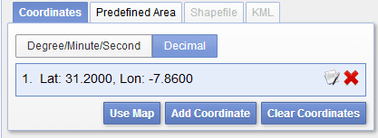
There are several ways to select data including, using the map and clicking a point, and/or drawing a rectangle over the area of interest. Alternatively, if you know the coordinates, you can use these by clicking the "Add Coordinate" button.
After inputting the coordinates, click the "Datasets >>" button to see the available data.
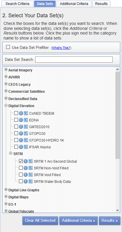
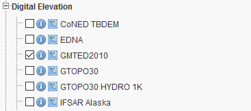
The SRTM DEMs can be found under the "Digital Elevation > SRTM" menu. You'll also notice that you can download GMTED2010 data here as well.
Select the "SRTM 1 Arc-Second Global" option, and then click the "Results >>" button.
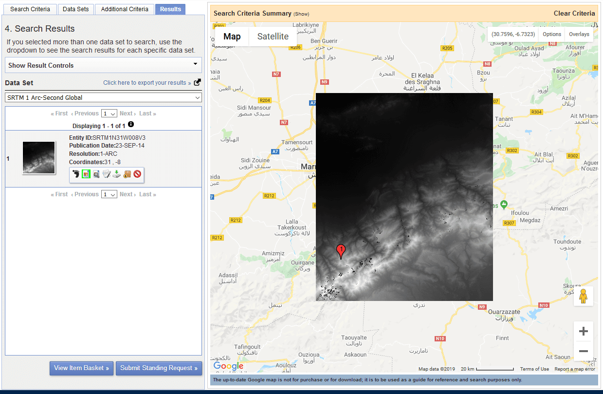
On the search results screen you'll be presented with the data matching the criteria you selected. Click the jpeg icon (highlighted green on the image above) to overlay the data on the map. If you are happy with the data, click the "Download options" icon (disk drive with a green arrow above it) to download the data.
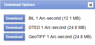
Select the GeoTiff option to download. When downloading DEMs, I would recommend you leave the file names as they are, as they contain useful information about the DEM tile.
To load this DEM in R, set the working directory to where you have saved the DEM file (for example "/R/maps/DEMs/"), and then use the following code:
# Load raster package
library(raster)
# Load SRTM DEM
ma.dem.SRTM <- raster("n31_w008_1arc_v3.tif")
If you downloaded a different grid square, change the file name in the above code. To plot the DEM, simply use plot():
plot(ma.dem.SRTM)
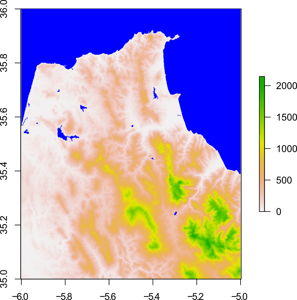
The following image is a comparison of the two downloaded SRTM DEM raster files (90 m vs. 30 m) plotted in R:
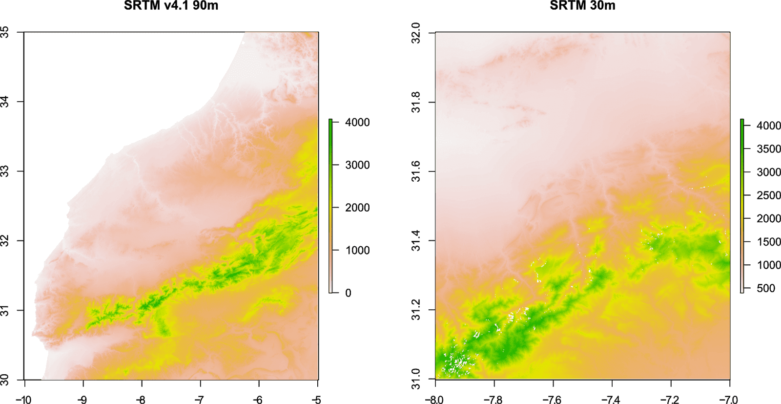
You'll notice the difference in resolution for the two files, and the missing data in the 30 m resolution DEM for our location in the High Atlas, Morocco. Other DEMs might be a better choice to represent our study area.
GMTED2010
| Horizontal datum | WGS84 |
| Vertical datum | EGM96 |
| Spatial resolution | ~1 kilometre (30 arc-seconds), ~500 metres (15 arc-seconds), ~250 metres (7.5 arc-seconds) |
| Format | GeoTiff |
| Raster size | 30° x 20° grid |
| Download | EarthExplorer (Requires registration) |
GMTED2010 or Global Multi-resolution Terrain Elevation Data 2010, is a replacement for the GTOPO30 DEM, created by the U.S. Geological Survey (USGS). This DEM is largely based on SRTM data, with other sources filling in the gaps for worldwide coverage.
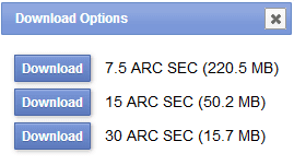
GMTED2010 is available at three spatial resolutions, with the 7.5 Arc-seconds providing the highest available resolution. To download the data, follow the steps for downloading SRTM data from the EarthExplorer, but select "GMTED2010" instead.
This will download a .zip file containing 7 GeoTiff images, which include DEMs containing: minimum elevation, maximum elevation, mean elevation, median elevation,standard deviation, systematic subsample, and breakline emphasis elevation data.
GMTED2010 is particularly useful if you want to compare minimum, maximum, and mean elevation data for a particular grid cell.
To load this DEM in R, set the working directory to where you have saved the DEM file, and then use the following code:
# Load raster package
library(raster)
# Load GMTED2010 DEM
ma.dem.GMTED.mean <- raster("GMTED2010N30W030_075/30n030w_20101117_gmted_mea075.tif") # Mean elevation
ma.dem.GMTED.min <- raster("GMTED2010N30W030_075/30n030w_20101117_gmted_min075.tif") # Min elevation
ma.dem.GMTED.max <- raster("GMTED2010N30W030_075/30n030w_20101117_gmted_max075.tif") # Max elevation
If you downloaded a different grid square, change the file and folder names in the above code. To plot the DEM, simply use plot().
You could also plot the mean, min and max elevations for our study area:
layout(matrix(1:3, ncol=3))
plot(ma.dem.GMTED.mean, xlim=c(-8, -7), ylim=c(31, 32))
plot(ma.dem.GMTED.min, xlim=c(-8, -7), ylim=c(31, 32))
plot(ma.dem.GMTED.max, xlim=c(-8, -7), ylim=c(31, 32))
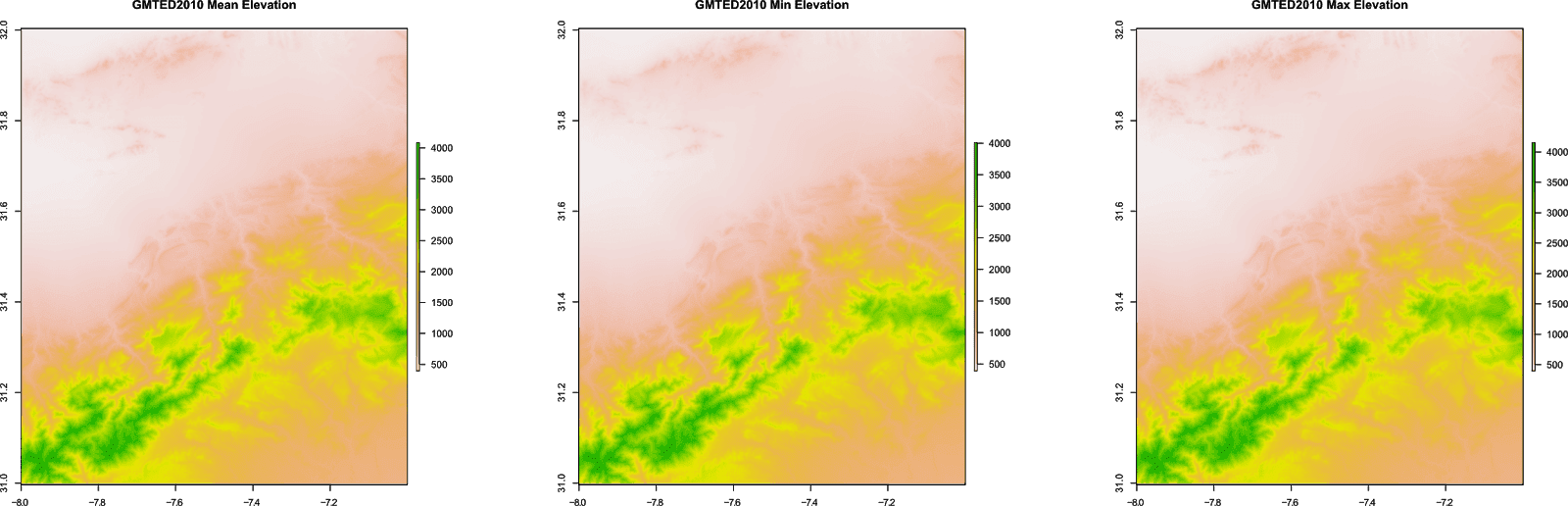
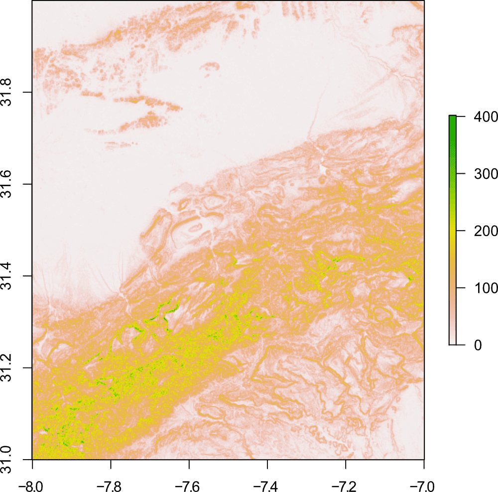
Can you spot the difference? No? (Click to enlarge). You can calculate the difference between the maximum and minimum elevations easily in R:
# Calculate difference between max/min elevation
ma.dem.GMTED.diff <- ma.dem.GMTED.max - ma.dem.GMTED.min
# Plot elevation difference
plot(ma.dem.GMTED.diff, xlim=c(-8, -7), ylim=c(31, 32))
ASTER
ASTER GDEM or Advanced Spaceborne Thermal Emission and Reflection Radiometer Global Digital Elevation Model, was created by NASA JPL and Japan's METI, and is now on version 3, offering improvements over previous versions of this DEM. A corresponding dataset: ASTER Water Body Dataset (ASTWBD), contains information on global water bodies including; oceans, rivers and lakes.
Data was collected by the ASTER instrument onboard NASA's Terra spacecraft using stereo-pairs of visible and near-infrared images. The DEM covers (almost) the entire world at ~30 metres resolution. Although some artefacts remain in the DEM, it is generally considered better than SRTM data, particularly for mountainous terrain.
ASTER GDEM V3
| Horizontal datum | WGS84 |
| Vertical datum | EGM96 |
| Spatial resolution | ~30 metres (1 arc-seconds) |
| Format | GeoTiff |
| Raster size | 1° x 1° grid |
| Download | NASA Earth Data (Requires registration) |
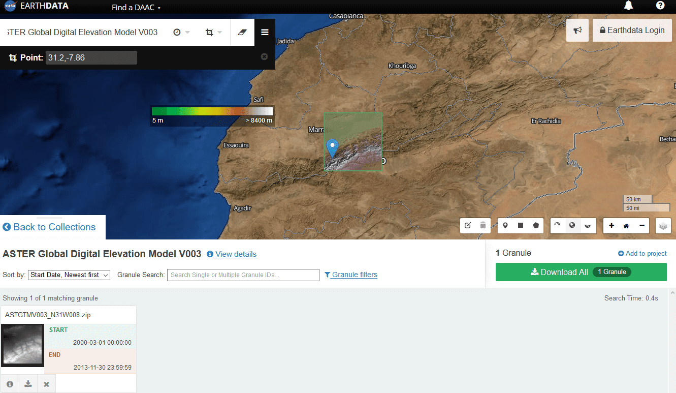
You can download the data from the NASA Earth Data, using "ASTER Global Digital Elevation Model V003" as the search term (see guide below).
ASTWBD
| Horizontal datum | WGS84 |
| Vertical datum | EGM96 |
| Spatial resolution | ~30 metres (1 arc-seconds) |
| Format | GeoTiff |
| Raster size | 1° x 1° grid |
| Download | NASA Earth Data (Requires registration) |
You can download the data from the NASA Earth Data, using "ASTER Global Water Bodies Database V001" as the search term (see guide below).
Downloading data using NASA Earth Data
Head to the NASA Earth Data website to download the data. You will need to register to be able to download data, although no registration is required to explore the datasets.
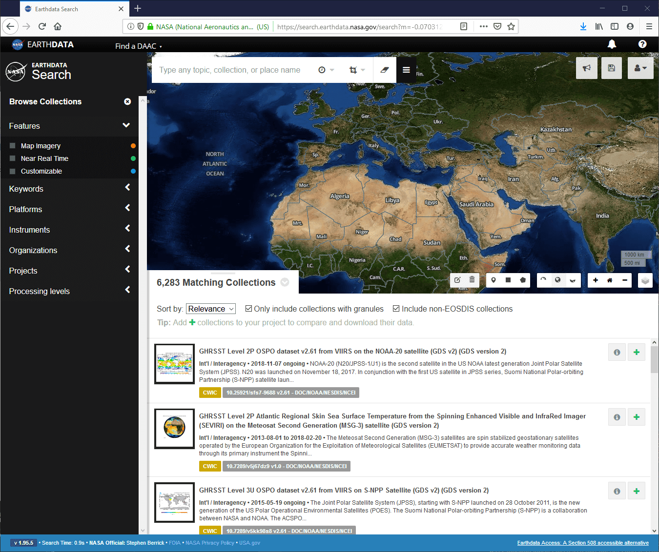
There are several ways to select data using the icons at the bottom of the map. The easiest way is to search by spatial coordinates.
After inputting the coordinates, you'll be presented with thousands of available datasets, so it is best to input the dataset you want into the search field.
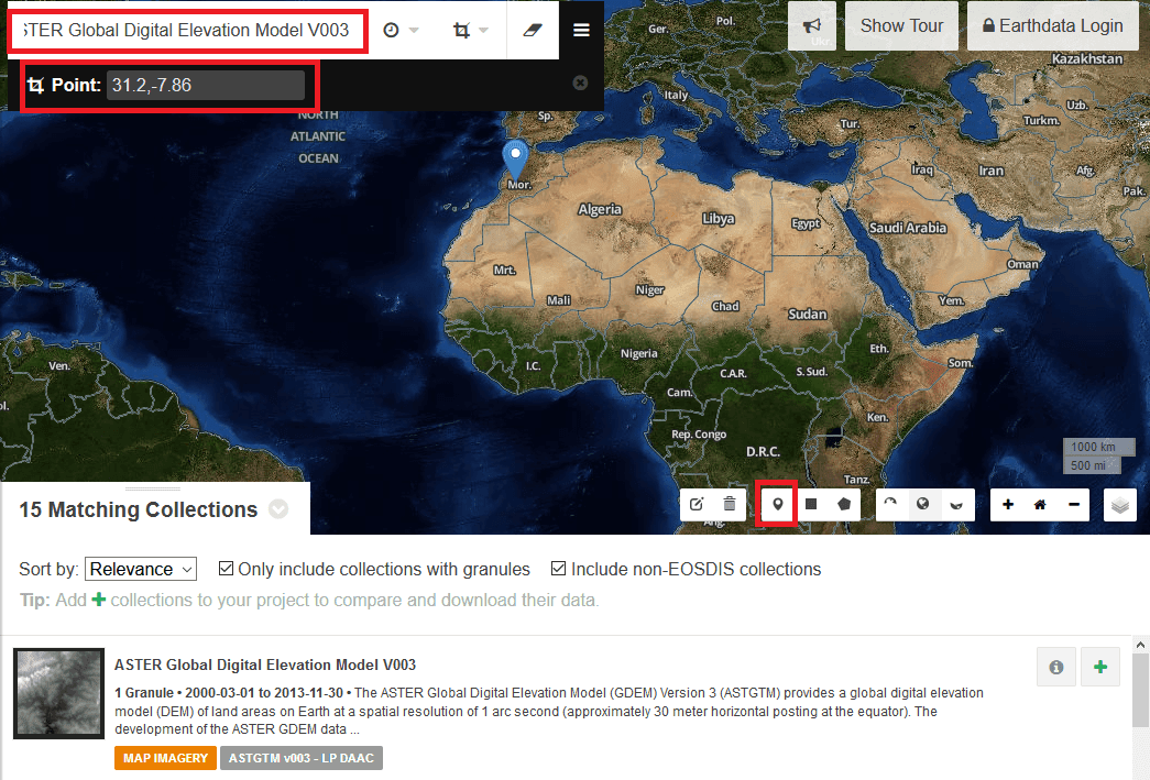
Searching for the "ASTER Global Digital Elevation Model V003" should present this as the first search result. There will also be many additional links to other ASTER data with similar names, so care should be taken to select the correct one. Click the link, where you'll see the available data for your coordinates and the option to download the file.
You'll need to be registered and logged in to download any data. Follow the instructions and links to download the data (there will be many!). The files will be downloaded as .zip files containing 2 GeoTiff images.
To load the DEM files in R, set the working directory to where you have saved the files, and then use the following code:
# Load raster package
library(raster)
# Load ASTER GDEM V3 DEM
ma.dem.ASTER <- raster("ASTGTMV003_N31W008/ASTGTMV003_N31W008_dem.tif")
# ASTER Water Body Dataset
ma.dem.ASTER.water <- raster("ASTWBDV001_N31W008/ASTWBDV001_N31W008_dem.tif")
If you downloaded a different grid square, change the file and folder names in the above code. To plot the DEM, simply use plot():
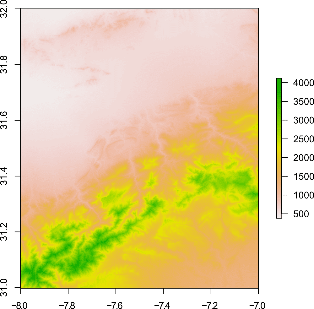
You could also overlay the Water Bodies data by using the following code:
# Plot DEM
plot(ma.dem.ASTER)
# Add water
plot(ma.dem.ASTER.water, zlim=c(0), col="blue", legend=FALSE, add=TRUE)
Clearly, this is not the best example, as only the Moulay Youssef Barrage water body is being picked up by the ASTER data.
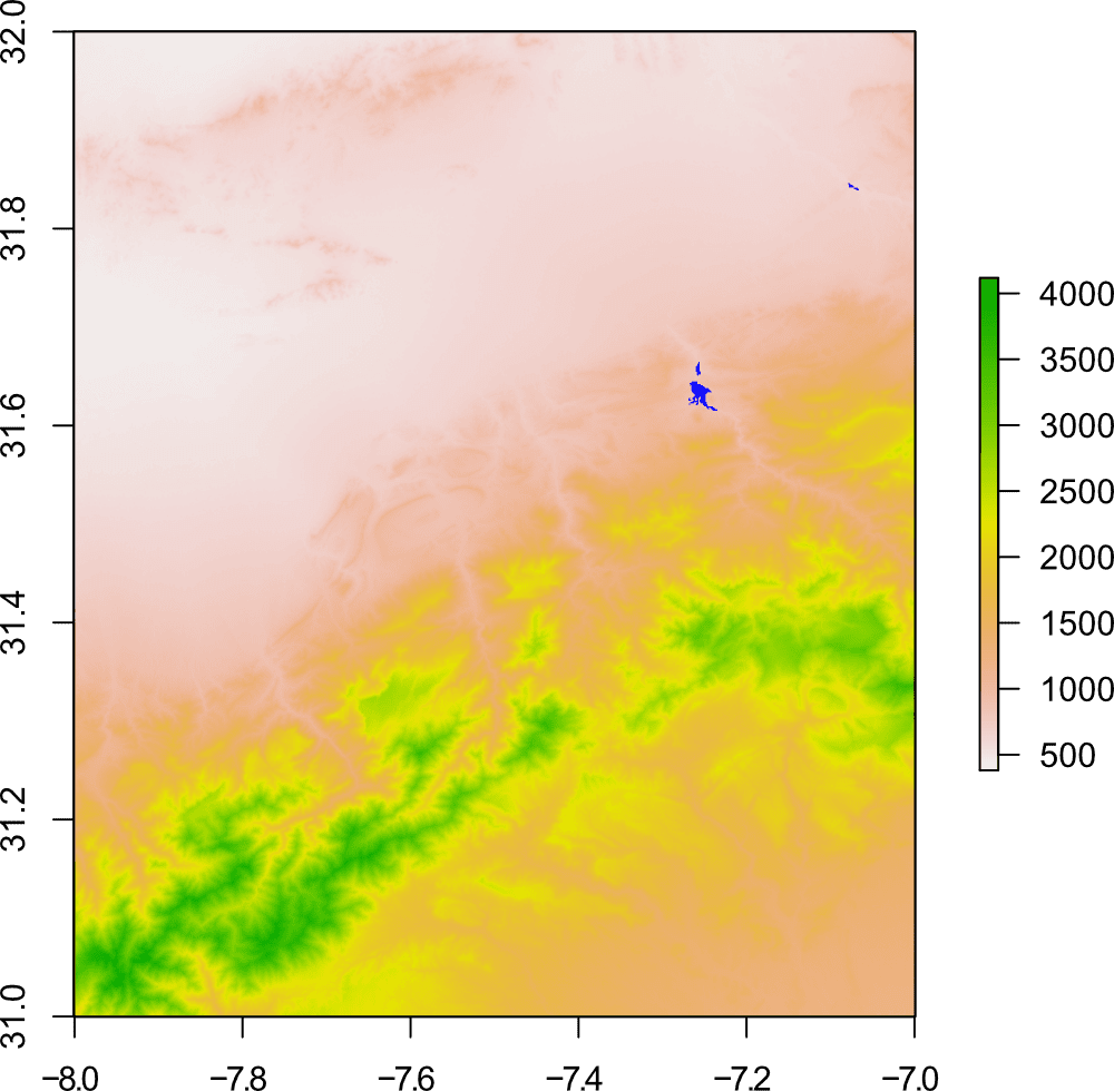
Here's another example from the north of Morocco near Tangier:
So, while the DEM has very good coverage, the Water Bodies dataset still requires some work, but it is useful for major water bodies.
ALOS World 3D
| Horizontal datum | WGS84 |
| Vertical datum | EGM96 |
| Spatial resolution | ~30 metres (1 arc-seconds) |
| Format | GeoTiff |
| Raster size | 1° x 1° grid |
| Download | ALOS World 3D Homepage (Requires registration) |
ALOS World 3D 30 m resolution (AW3D30) is a free version of the commercial ALOS World DEM (5 m resolution), created by Japan Aerospace Exploration Agency (JAXA).
Data is collected by the Panchromatic Remote-sensing Instrument for Stereo Mapping (PRISM) onboard the Advanced Land Observing Satellite "DAICHI". The radiometer collects three independent images (nadir, backwards, and forwards), and produces a stereoscopic image of the Earth's surface from which the DEM is created.
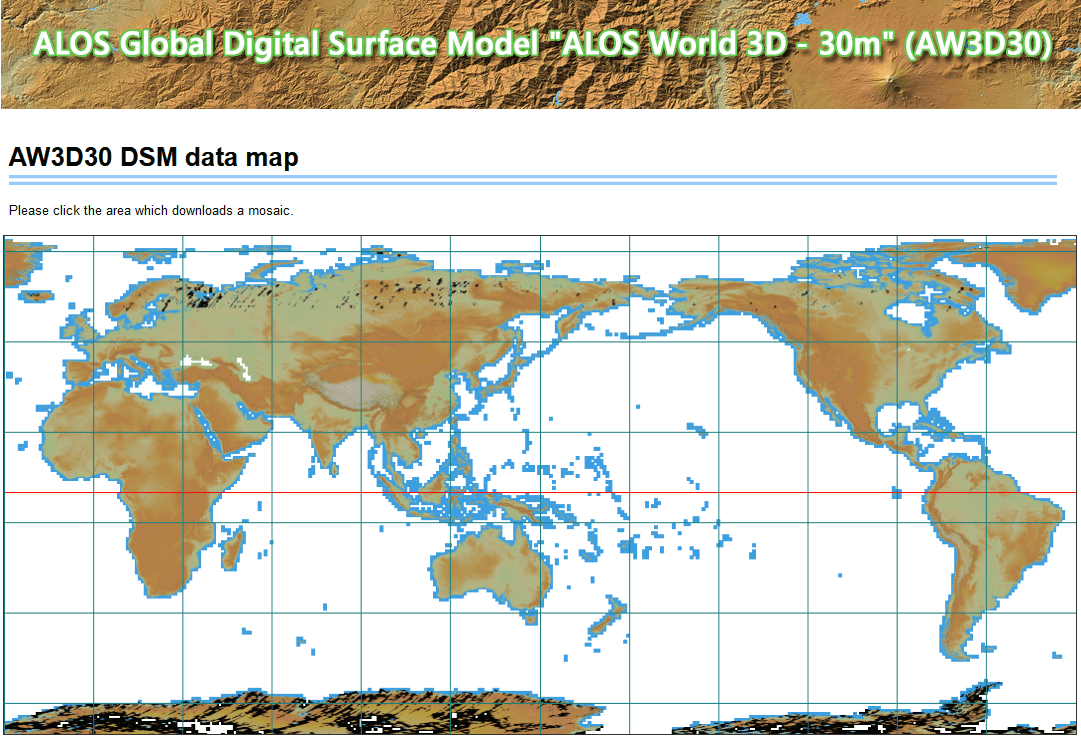
ALOS World 3D has near worldwide coverage. To download, head to the ALOS World 3D Homepage. Before you can access the data, you will need to register.
Once registered, you can use the download link and input your username and password when prompted.
You'll be presented with a map of the world, click the relevant part to select data:
Continue clicking though the map:
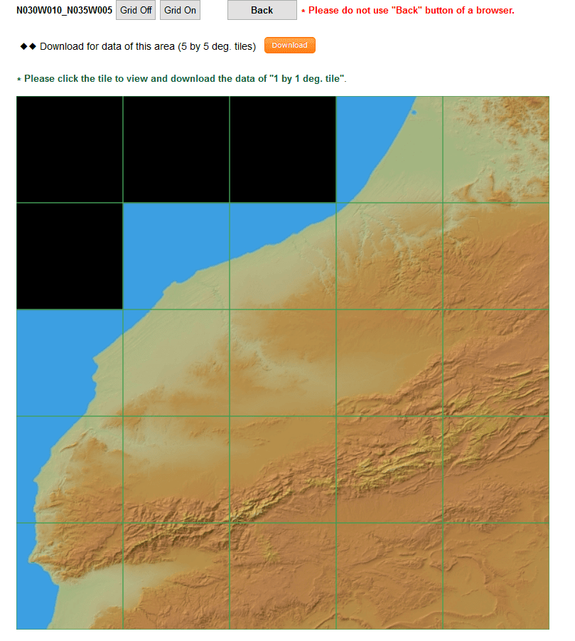
You can either download all the tiles on this page (5° x 5°), or click through again to the relevant tile (1° x 1°).
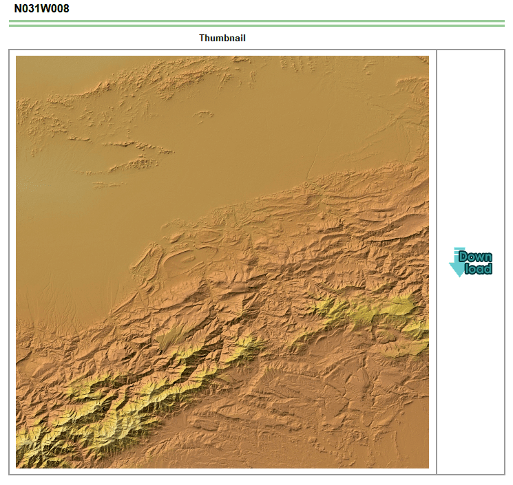
The DEM will be downloaded as a .tar.gz file. Extract the DEM using 7-Zip. If you downloaded the 5° x 5° data, you will have a folder with multiple 1° x 1° DEM tiles.
If you downloaded the 1° x 1°, there will be 3 GeoTiff files and 3 .txt files. The file named "N031W008_AVE_DSM.tif" contains the DEM.
To load this DEM in R, set the working directory to where you have saved the DEM file, and then use the following code:
# Load raster package
library(raster)
# Load ALOS World 3D DEM
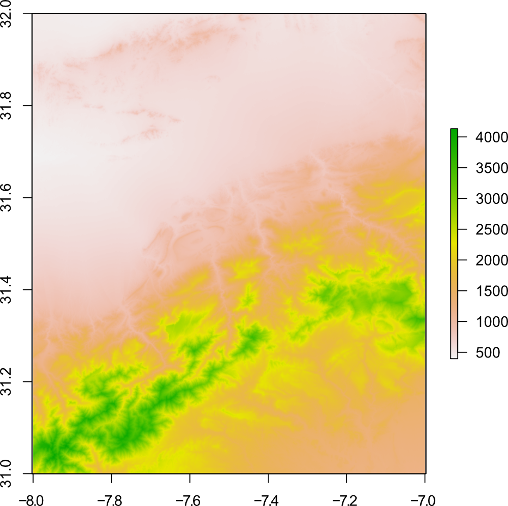
ma.dem.ALOS <- raster("N031W008/N031W008_AVE_DSM.tif")
If you downloaded a different grid square, change the file and folder names in the above code. To plot the DEM, simply use plot().
DEM Comparison
Now that we have downloaded several DEMs, lets compare them! First, we'll compare them using the grid size 0.2° x 0.2°.
You can do this yourself using the following code:
layout(matrix(1:6, ncol=3))
plot(ma.dem.SRTM90, xlim=c(-8, -7.8), ylim=c(31, 31.2), main="SRTM v4.1 90m")
plot(ma.dem.SRTM, xlim=c(-8, -7.8), ylim=c(31, 31.2), main="SRTM 30m")
plot(ma.dem.GMTED.mean, xlim=c(-8, -7.8), ylim=c(31, 31.2), main="GMTED2010 Mean")
plot(ma.dem.ASTER, xlim=c(-8, -7.8), ylim=c(31, 31.2), main="ASTER GDEM V3")
plot(ma.dem.ALOS, xlim=c(-8, -7.8), ylim=c(31, 31.2), main="ALOS World 3D")
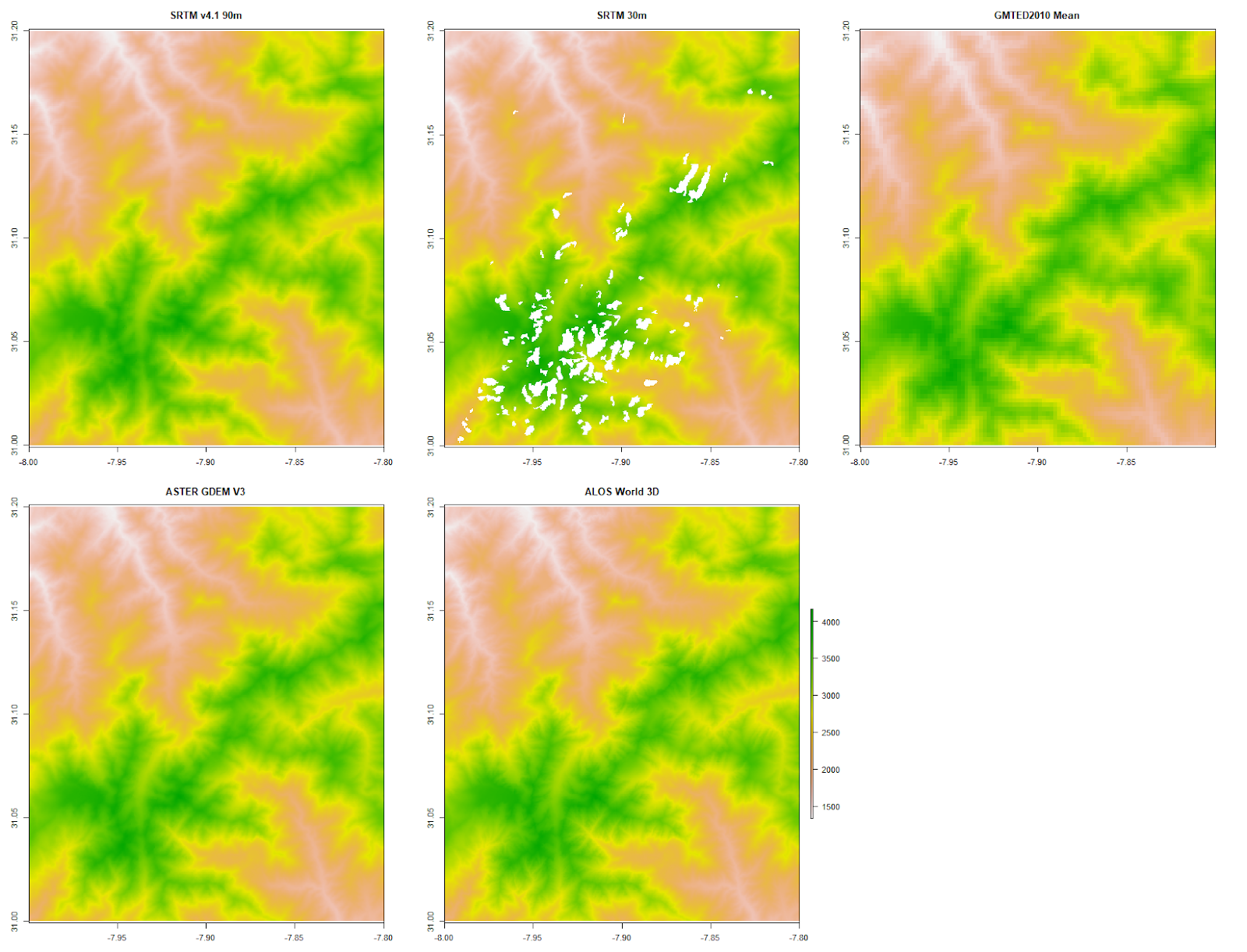
You can start to see some pixilation in the GMTED2010 DEM, while the other DEMs still look okay, except for the missing data in SRTM 30 m. (Click image to enlarge).
Let's zoom in to 0.05° x 0.05°:
layout(matrix(1:6, ncol=3))
plot(ma.dem.SRTM90, xlim=c(-8, -7.95), ylim=c(31, 31.05), main="SRTM v4.1 90m")
plot(ma.dem.SRTM, xlim=c(-8, -7.95), ylim=c(31, 31.05), main="SRTM 30m")
plot(ma.dem.GMTED.mean, xlim=c(-8, -7.95), ylim=c(31, 31.05), main="GMTED2010 Mean")
plot(ma.dem.ASTER, xlim=c(-8, -7.95), ylim=c(31, 31.05), main="ASTER GDEM V3")
plot(ma.dem.ALOS, xlim=c(-8, -7.95), ylim=c(31, 31.05), main="ALOS World 3D")
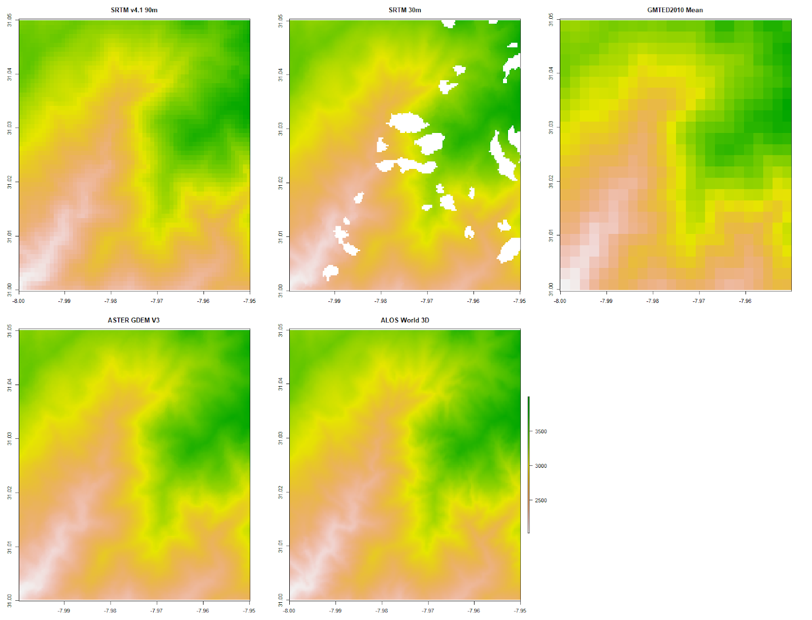
The pixilation in the GMTED2010 DEM is now very obvious, and is becoming evident in the SRTM v4.1 90 m DEM. The missing data in the SRTM 30 m DEM remains a problem. (Click image to enlarge).
Let's zoom in to 0.01° x 0.01° for our final comparison:
layout(matrix(1:6, ncol=3))
plot(ma.dem.SRTM90, xlim=c(-8, -7.95), ylim=c(31, 31.05), main="SRTM v4.1 90m")
plot(ma.dem.SRTM, xlim=c(-8, -7.95), ylim=c(31, 31.05), main="SRTM 30m")
plot(ma.dem.GMTED.mean, xlim=c(-8, -7.95), ylim=c(31, 31.05), main="GMTED2010 Mean")
plot(ma.dem.ASTER, xlim=c(-8, -7.95), ylim=c(31, 31.05), main="ASTER GDEM V3")
plot(ma.dem.ALOS, xlim=c(-8, -7.95), ylim=c(31, 31.05), main="ALOS World 3D")
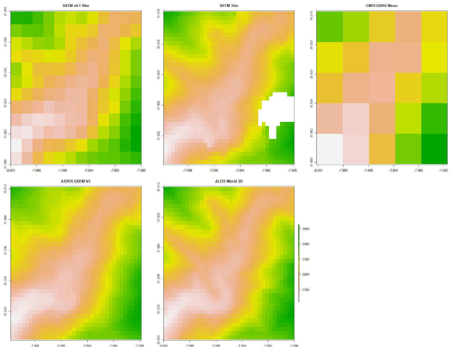
In terms of detail, it looks like the ALOS World 3D DEM may just have edged it against the ASTER GDEM V3 DEM. Of course, your results may vary for different areas. (Click image to enlarge).
Thanks for reading, and please leave any comments or questions below.
Further reading
Creating simple location maps in R - A guide to show you how to create simple location maps (a large overview, an small study area map), including adding points of interest, grids, scale bars and north arrows. No GIS skills needed!
Bathymetric maps in R: Getting and plotting data - Part 1 of a guide showing how and where to get bathymetry data and how to import it into R.Bathymetric maps in R: Colour palettes and break points - Part 2 of the bathymetry guide taking an in-depth look at colour schemes for raster plots.
A quick guide to pch symbols - A quick guide to the different pch symbols which are available in R, and how to use them. [R Graphics]
A quick guide to layout() in R - How to create multi-panel plots and figures using the layout() function. [R Graphics]
Interpolating gridded datasets in R: UV-B data - How to interpolate gridded datasets and plot them in R.
No comments
Post a Comment
Comments are moderated. There may be a delay until your comment appears.